A 2D MHD Problem: The Orszag-Tang vortex

To run an example 2D MHD problem, follow these steps.

Clean up any old files from the last compilation, configure, and compile
```
 % make clean
 % configure --with-problem=orszag-tang --with-order=3
 % make all
```
Note we increased the order of the spatial reconstruction to 3 in this example.
Run the code using the default input file for the Orszag-Tang vortex
```
 % cd bin
 % athena -i ../tst/2D-mhd/athinput.orszag-tang
```
Once again, the code will print information about each time step, and finish with diagnostic information. The last few lines of output generated while the code was running should look something like the following
```
 cycle=655 time=9.999868e-01 next dt=1.320914e-05 last dt=1.449403e-03
 cycle=656 time=1.000000e+00 next dt=0.000000e+00 last dt=1.320914e-05
    
 terminating on time limit
   tlim= 1.000000e+00   nlim= 100000
   time= 1.000000e+00  cycle= 656
    
 zone-cycles/cpu-second = 2.403616e+05
    
 elapsed wall time = 1.006279e+02 sec.
    
 zone-cycles/wall-second = 2.403189e+05
 Global min/max for P: 0.0100164 0.755822
 Global min/max for d: 0.0442782 0.609765
    
 Simulation terminated on Thu Apr 29 10:02:04 2010
```
The exact numbers may change on different systems. The zone-cycles/cpu-second is a measure of performance: how many cells the code updated per cpu second. For 2D MHD, several hundred thousand is typical. Note the code took much longer to run (about 100 seconds) compared to the 1D hydro tests, because 2D MHD is much more work. The global min/max are the maximum and minimum values over the whole evolution for the variables being output (the pressure P and density d in this case).
When it finishes, the code should have produced a large number of output files (too many to list), with names OrszagTang.*.d.ppm, OrszagTang.*.P.ppm, OrszagTang.*.bin, and OrszagTang.hst. The *.ppm files are images of the density and pressure. The *.bin files are binary dumps of all variables. Finally, the OrszagTang.hst file is a formatted table with the time history of various variables.
Try making an animation of the image files. The easiest way is using ImageMagick routines.
```
 % animate *.d.ppm
```
An animation of the density should appear on your screen. You can also try animating the image files using IDL or MatLab; there are example scripts and .m files in /athena/vis that might help. Try animating the pressure as well.

The *.bin files contain unformatted writes of floating-point values for all the dependent variables.
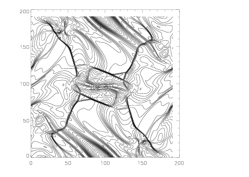
They can be read with, for example, the IDL script /athena/vis/idl/pltath.pro. If you have IDL on your system, try making a contour plot of the density using the following

 % idl
 IDL> .r ../vis/idl/pltath.pro
 % Compiled module: READBIN.
 % Compiled module: FOUR_PLOT.
 % Compiled module: NINE_PLOT.
 % Compiled module: SOD_PLOT.
 % Compiled module: FLINES.
 % Compiled module: READVTK.
 % Compiled module: MATCHSECHEAD.
 % Compiled module: READVECTBLOCK.
 % Compiled module: READSCALARBLOCK.
 IDL> readbin,'OrszagTang.0050.bin'
 IDL> contour,d,nlevels=30,/isotropic

You should see the following plot on your screen:

alt ot

By default, the binary dumps contain the conserved variables. The IDL script used above automatically computes the primitive variables (e.g. velocity instead of momentum density). To dump the primitive variables instead, the input file must be modified to include the line
```
 out   = prim
```
in the <output> block that generates the bin files. How to do this is described in more detail on the next page (Editing the Input File).
The OrszagTang.hst file contains a formatted table with the time-evolution (history) of various quantities.
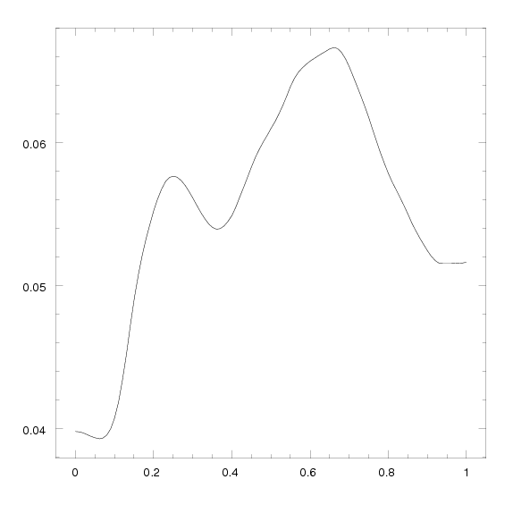
The data can be plotted with sm, IDL, MatLab, etc. If you have sm, try plotting the history of the magnetic energy using the following
```
 % sm
 Hello James, please give me a command
 : data OrszagTang.hst
 : read {t 1 mex 11 mey 12 mez 13}
 Read lines 1 to 103 from OrszagTang.hst
 : set me=mex+mey+mez
 : limits t me
 : device x11
 : box
 : connect t me
```
You should see the following plot of the time history of the total magnetic energy on your screen.

There are many more 2D hydrodynamics and MHD problems you can try running, the ApJS Method Paper describes many of them. In the next two sections of this Tutorial, we will describe how to control the properties of Athena calculations using parameters in the input file, and through the command line interface.