A 3D MHD Problem: The Rayleigh-Taylor Instability

To run an example 3D MHD problem, follow these steps.

Clean up any old files from the last compilation, configure, and compile

 % make clean
 % configure --with-problem=rt --with-order=3
 % make all

Run the code using the default input file. Because 3D problems are very expensive, it is wise to reduce the grid resolution if you are running on a single processor. This can be done using the command line.
```
 % cd bin
 % athena -i ../tst/3D-mhd/athinput.rt domain1/Nx1=32 domain1/Nx2=32 domain1/Nx3=64 time/tlim=3.0
```
Even at this reduced resolution, the run will take close to an hour to complete. Doubling the resolution in each dimension increases the run time in 3D by $2^4=16$ (a factor of 2 for each dimension, plus a factor of 2 for the smaller timestep), so if the default grid resolution specified in the input file is used, this test will take upwards of 12 hours to run (these numbers depend on the processor you are using of course). At low resolution, the bubbles (fingers) tend to rise (sink) faster, so the run is terminated at t=3 before they hit the top and bottom of the domain.

The last few lines output by the code should look like the following.

 cycle=3004 time=2.999249e+00 next dt=7.514237e-04 last dt=8.588881e-04
 cycle=3005 time=3.000000e+00 next dt=0.000000e+00 last dt=7.514237e-04
    
 terminating on time limit
   tlim= 3.000000e+00   nlim= 100000
   time= 3.000000e+00  cycle= 3005
    
 zone-cycles/cpu-second = 9.878593e+04
    
 elapsed wall time = 1.993715e+03 sec.
    
 zone-cycles/wall-second = 9.877826e+04
 Global min/max for d: 0.944639 10.1421
    
 Simulation terminated on Thu Apr 29 14:02:09 2010

Note the zone-cycles/cpu-second is significantly decreased in 3D compared to 2D MHD, by about a factor of 2.5. This is due to all the extra work required per cell in 3D, and poorer cache performance due to larger data structures.

The run should have generated ppm images of the density. Try using ImageMagick to make a movie of the density.
```
 % animate *.d.ppm
```
The images are made from a 2D slice in the X-Z plane, and therefore motion in Y makes features appear and disappear.
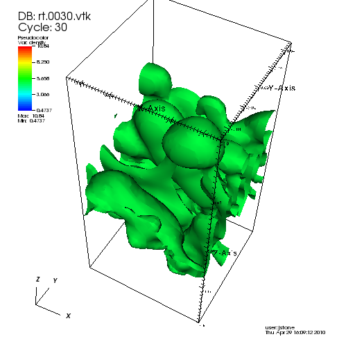
The code will also have generated a series of vtk files. An advantage of vtk files with 3D simulations is that VisIt, which has extensive visualization capabilities for 3D data, can read Athena vtk files directly. For example, by making an isosurface plot of the density with one level at the end of the calculation (select and Open rt.0030.vtk, choose Plot=pseudocolor of density, Operators=isosurface, OpAtts=isosurface, Select by Values with a single level at 5.0), you should see the following (after the appropriate rotation)
Try plotting other variables, such as the vertical velocity, from this test using VisIt or any other graphics package you like.
There are many other hydrodynamic and MHD problems that can be run in 3D: the problem generators for each are in /athena/src/prob, and the input files are in /athena/tst/3D-hydro and /athena/tst/3D-mhd. Try running some other problems, for example the hydrodynamic blast wave test.