Running Athena with SMR

Documentation/Tutorial/Athena with SMR

A powerful capability in Athena is the use of static (or fixed) mesh refinement (SMR). SMR is most useful when the problem consists of fixed regions where small length scales must be resolved, for example the midplane of an accretion disk, the center of a cluster of galaxies, or the beam of a supersonic jet. SMR is far more efficient on parallel processors than adaptive mesh refinement (AMR), enabling much larger, better resolved simulations.

The use of SMR is complex, however as an introduction to this capability, follow these steps to run a 2D version of the MHD Rayleigh-Taylor instability problem.

Clean up any old files from the last compilation, enable SMR during configure, and compile.
```
 % make clean
 % configure --with-problem=rt --with-order=3 --enable-smr
 % make all
```
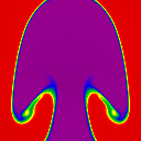
SMR grids are defined using multiple <domain> blocks in the input file. The total number of blocks to be read is controlled by the num_domains parameter in the <job> block. First, try running the 2D MHD RT problem using a single (root level) grid using the default input file
```
 % cd bin
 % athena -i ../tst/2D-mhd/athinput.rt time/tlim=4.0
```
When the code finishes, there should be a number of vtk files, and images of the density, produced. The final image of the density should look like the following:
Now rerun the problem with 2 levels of refinement. The default input file specifies a root grid with resolution 64x128, plus a level=1 Domain with resolution 128x128 that spans the center of the root level. To run the code with two levels, use
```
 % athena -i ../tst/2D-mhd/athinput.rt time/tlim=4.0 job/num_domains=2
```
With SMR, the code outputs data to different directories for levels>0. The root (level=0) Domain will output files to the directory in which the code was run (or specified by the -d command line option), while the level=1 Domain outputs data to a new directory called lev1. Images of the density in the root and level=1 directories at t=4 should look like the following.

The root level image uses the fine grid solution where the two overlap, so the central regions are slightly different than the plot shown above for a single grid (step 2). The interface is sharper, and there is less mixing, on the higher resolution (level=1) grid.

Also note that each Domain also creates its own history file; try plotting the time-evolution of various quantities in the root and level=1 Domains. Quantities are not conserved in the latter, because fluid can flow through fine/coarse boundaries.
The location of higher-level Domains in the root level is specified by the iDisp, jDisp, and kDisp parameters in the corresponding <domain> block. These are the displacement of the Domain from the left-edge in each dimension, measured in units of grid cells at that level. For the example above, iDisp=0 and jDisp=64, which means the level=1 Domain touches the left and right sides of the root level in the x1-direction, and is centered in the x2-direction. Try running a problem where jDisp=96. Then try running a problem where the level=1 Domain has dimensions 64^2^, and is centered in both the x1- and x2-directions (this would require iDisp=32 and jDisp=96).
Try adding additional Domains with higher resolution by adding new <domain> blocks to the input file, and increasing num_domains appropriately. For each level you add, a new lev* directory which contains the data for that level will be created.
Running SMR with MPI gets even more complicated. Now, each id* directory created by each processor will contain a hierarchy of lev* directories. Some directories will be empty if the processor that created it does not contain a Grid on that level.

Once you are running SMR with MPI, you are becoming an expert user, and you should consult the User Guide to learn more.