A 1D Hydrodynamics Problem: The Sod shocktube
Documentation/Tutorial/1D Hydro
To run a simple 1D hydrodynamics problem, follow these steps.
-
Clean up any old files from the last compilation.
% make clean -
Configure the code for hydrodynamics and the shock tube problem generator
% configure --with-gas=hydro --with-problem=shkset1dConfigure will echo lots of diagnostic messages, and output a summary of the configuration options.
-
Compile. This will create the
/bindirectory, if it does not already exist.% make all -
Run the code using the default input file for the Sod shocktube
 % cd bin
 % athena -i ../tst/1D-hydro/athinput.sod
The code will print information about each time step, and finish with diagnostic information like zone-cycles/second.
-
The code should have produced a series of .tab files, and a history file:
 % ls
 athena        Sod.0005.tab  Sod.0011.tab  Sod.0017.tab  Sod.0023.tab
 Sod.0000.tab  Sod.0006.tab  Sod.0012.tab  Sod.0018.tab  Sod.0024.tab
 Sod.0001.tab  Sod.0007.tab  Sod.0013.tab  Sod.0019.tab  Sod.0025.tab
 Sod.0002.tab  Sod.0008.tab  Sod.0014.tab  Sod.0020.tab  Sod.hst
 Sod.0003.tab  Sod.0009.tab  Sod.0015.tab  Sod.0021.tab
 Sod.0004.tab  Sod.0010.tab  Sod.0016.tab  Sod.0022.tab
The .tab files are formatted tables of the dependent variables output every 0.01 in problem time (the type and frequency of outputs are set by parameters in the input file).
-
To plot the data in one of the .tab files, your favorite graphics package can be used. For example, to plot the density (3rd column in the file) using SuperMongo (
smmust be installed on your system), use% sm Hello James, please give me a command : data Sod.0025.tab : read {x 1 d 3} : Read lines 1 to 132 from Sod.0025.tab : limits x d : device x11 : box : points x dYou should now see the following plot on the screen:
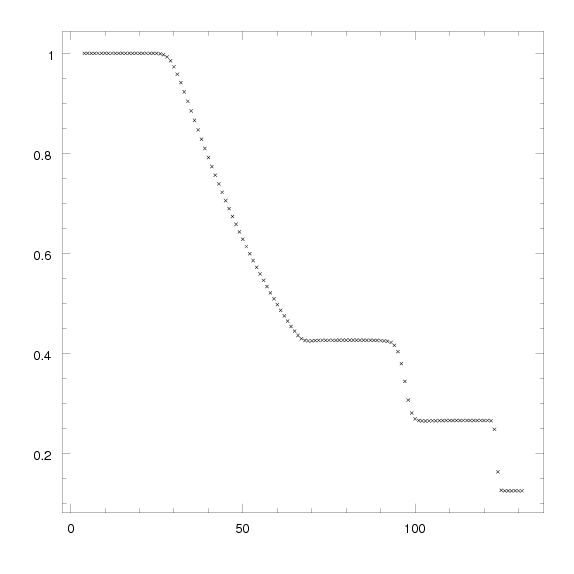
Of course, any graphics package you like (IDL, MatLab, etc.) can be used to plot the data.
-
Try plotting other variables (other columns in the .tab file), and variables at other times (other .tab files).
You can also try making a movie by reading all the .tab files and making plots using the data in each file.
The problem you’ve just run is an example of a Riemann, or shocktube, problem. More details about this particular problem are given on the Tests: section, and in the Method Papers (in particular, see the ApJS method paper).
These links also describe many more 1D hydrodynamic tests that can be run. However, the next step in this Tutorial (see next section) is a 2D MHD problem.