DESCUR
The DESCUR code calculates a set of Fourier Harmonics which describe some closed toroidal surface.
Theory
The DESCUR code uses a steepest descent algorithm to find a least-squares approximation to an arbitrary 3D space curve. Angle constraints, based on a minimum spectral width criterion, are applied. The constrain is satisfied by tangential variations along the curve.
Compilation
The code is part of the STELLOPT package.
Input Data Format
The code is interactive prompting the user for input. The spectral convergence parameter, representation, and source data are input from the command line. Source data can be specified as a series of R, phi, Z points in a test file, Fourier coefficients from a text file or VMEC output (wout file), a Solove've equilibrium, ellipse, D-shape, bean, belt, square or heliac. If fitting a set of R-phi-Z points the code expects the first line to be contain the number of points in theta, the number of points in phi and the periodicity of the boundary. The subsequent lines contain the R, phi, and Z coordinates in theta then phi order as so:
24  24  3
1.5  0.0  0.00
1.4  0.0  0.20
1.3  0.0  0.50
1.2  0.0  0.55
1.1  0.0  0.60
 .    .    .
 .    .    .
 .    .    .
If fitting an axisymmetric surface then the following formulation may be used where only R and Z are specified.
24  1  3
1.5  0.00
1.4  0.20
1.3  0.50
1.2  0.55
1.1  0.60
 .    .
 .    .
 .    .
If reading VMEC output either the WOUT file may be passed to DESCUR when prompted or a file with a set of Fourier harmonics. If the Fourier harmonics are passed the first line of the file should have MPOL, NPHI, and NFP specified on the first line, subsequent lines should have n,m, r-cosine, and z-sine as so:
0  5  1
0  0  1.0  0.0
0  1  0.5  0.5
0  2  0.1  0.0
.  .   .    .
.  .   .    .
.  .   .    .
Execution
The code runs interactively as so:
>~/bin/xcurve
 Enter spectral convergence parameter
 = 0 for polar,  = 1 for equal arclength
 >1 for smaller spectral width
 = 4 corresponds to STELLOPT choice): 4
 Use (default) VMEC-compatible compression (V)
 or Advanced Hirshman-Breslau compression (A): V
 Select source of curve data to be fit:
 0 :  Points from file
 1 :  Fourier coeffs from file (wout file allowed)
 2 :  Solove'ev Equilibrium
 3 :  Assorted 2-D shapes

3
  Shape to fit: 1=ellipse; 2=D; 3=bean; 4=belt; 5=square; 6=heliac)
3
 ORDERING SURFACE POINTS
 Average elongation = 1.2850E+00
 Raxis =   3.0000E+00 Zaxis =  -6.4514E-17
 Number of Theta Points Matched =   400
 Number of Phi Planes =     1
 Max Poloidal Mode Number =    19
 Max Toroidal Mode Number =     1

                  Fitting toroidal plane #   1

 RAXIS =  3.000E+00 ZAXIS = -6.451E-17 R10 =  1.697E+00

 ITERATIONS    RMS ERROR    FORCE GRADIENT    <M>    MAX m   DELT
       1       1.604E-02       8.625E-04      1.66      19  9.70E-01
     100       3.179E-05       2.417E-05      1.69      19  9.70E-01
     114       1.161E-05       8.099E-06      1.69      19  9.70E-01

 ANGLE CONSTRAINTS WERE APPLIED
 BASED THE POLAR DAMPING EXPONENT (PEXP) =  4
 RM**2 + ZM**2 SPECTRUM COMPUTED WITH P =     4.00 AND Q =     1.00
 TIME:   6.21E-02 SEC.

  OUTPUTTING FOURIER COEFFICIENTS TO OUTCURVE FILE

 Do you wish to plot this data (Y/N)? N
Output Data Format
Two output data files are produced, an 'outcurve' and an 'plotout' file. The 'outcurve' contains the runtime output of the code and the Fourier harmonics at it's end
 Average elongation = 1.2850E+00
 Raxis =   3.0000E+00 Zaxis =  -6.4514E-17
 Number of Theta Points Matched =   400
 Number of Phi Planes =     1
 Max Poloidal Mode Number =    19
 Max Toroidal Mode Number =     1

                  Fitting toroidal plane #   1

 RAXIS =  3.000E+00 ZAXIS = -6.451E-17 R10 =  1.697E+00

 ITERATIONS    RMS ERROR    FORCE GRADIENT    <M>    MAX m   DELT
       1       1.604E-02       8.625E-04      1.66      19  9.70E-01
     100       3.179E-05       2.417E-05      1.69      19  9.70E-01
     114       1.161E-05       8.099E-06      1.69      19  9.70E-01

 ANGLE CONSTRAINTS WERE APPLIED
 BASED THE POLAR DAMPING EXPONENT (PEXP) =  4
 RM**2 + ZM**2 SPECTRUM COMPUTED WITH P =     4.00 AND Q =     1.00
 TIME:   6.21E-02 SEC.


   MB  NB      RBC         RBS         ZBC         ZBS        RAXIS       ZAXIS
    0   0  2.9768E+00  0.0000E+00  1.2371E-16  0.0000E+00  3.0000E+00  0.0000E+00
    1   0  1.0279E+00  5.1324E-17  5.1324E-17  1.3589E+00
    2   0  5.0840E-01 -4.8835E-17 -4.5683E-17  2.9345E-01
    3   0 -1.7459E-02  9.3551E-18  8.0878E-18  1.3372E-02
    4   0  1.2897E-02 -4.3181E-17 -3.7274E-17  5.3717E-04
    5   0 -5.1679E-03  6.7965E-17  6.5705E-17  1.1723E-03
    6   0  2.8280E-03 -5.9904E-17 -4.4011E-17 -3.8643E-04
    7   0 -1.6359E-03  4.2172E-17  7.3761E-18 -1.4547E-05
    8   0  8.8040E-04 -1.5332E-18  3.1346E-17  1.3665E-04
    9   0 -4.4860E-04 -2.1453E-18 -2.0277E-17 -1.4472E-04
   10   0  2.0444E-04  3.6793E-17  2.4582E-17  1.0020E-04
   11   0 -8.2919E-05  2.3427E-17  3.3476E-17 -5.3261E-05
   12   0  2.8419E-05  7.2167E-19 -2.8877E-17  2.1852E-05
   13   0 -6.3884E-06 -1.9872E-17 -4.9042E-17 -8.8152E-06
   14   0 -1.4092E-06 -3.5350E-17 -2.0153E-17  4.9542E-06
   15   0  3.1699E-06 -5.7647E-17 -1.8769E-17 -1.8008E-06
   16   0 -1.7898E-06 -1.7439E-17  1.5097E-17 -1.9403E-06
   17   0 -1.4764E-07 -2.8074E-17  1.8244E-17  3.1605E-06
   19   0 -1.0601E-06 -3.1500E-18  3.1500E-18 -1.0601E-06

  RBC(0,0) =   2.976759E+00   RBS(0,0) =   0.000000E+00   ZBC(0,0) =   1.237137E-16   ZBS(0,0) =   0.000000E+00
  RBC(0,1) =   1.027882E+00   RBS(0,1) =   5.132439E-17   ZBC(0,1) =   5.132439E-17   ZBS(0,1) =   1.358919E+00
  RBC(0,2) =   5.083998E-01   RBS(0,2) =  -4.883497E-17   ZBC(0,2) =  -4.568290E-17   ZBS(0,2) =   2.934464E-01
  RBC(0,3) =  -1.745890E-02   RBS(0,3) =   9.355075E-18   ZBC(0,3) =   8.087806E-18   ZBS(0,3) =   1.337203E-02
  RBC(0,4) =   1.289742E-02   RBS(0,4) =  -4.318108E-17   ZBC(0,4) =  -3.727371E-17   ZBS(0,4) =   5.371726E-04
  RBC(0,5) =  -5.167947E-03   RBS(0,5) =   6.796532E-17   ZBC(0,5) =   6.570472E-17   ZBS(0,5) =   1.172259E-03
  RBC(0,6) =   2.827957E-03   RBS(0,6) =  -5.990360E-17   ZBC(0,6) =  -4.401130E-17   ZBS(0,6) =  -3.864267E-04
  RBC(0,7) =  -1.635860E-03   RBS(0,7) =   4.217155E-17   ZBC(0,7) =   7.376138E-18   ZBS(0,7) =  -1.454712E-05
  RBC(0,8) =   8.804028E-04   RBS(0,8) =  -1.533169E-18   ZBC(0,8) =   3.134615E-17   ZBS(0,8) =   1.366483E-04
  RBC(0,9) =  -4.486042E-04   RBS(0,9) =  -2.145350E-18   ZBC(0,9) =  -2.027734E-17   ZBS(0,9) =  -1.447159E-04
  RBC(0,10) =   2.044422E-04   RBS(0,10) =   3.679311E-17   ZBC(0,10) =   2.458171E-17   ZBS(0,10) =   1.001997E-04
  RBC(0,11) =  -8.291926E-05   RBS(0,11) =   2.342734E-17   ZBC(0,11) =   3.347551E-17   ZBS(0,11) =  -5.326074E-05
  RBC(0,12) =   2.841938E-05   RBS(0,12) =   7.216676E-19   ZBC(0,12) =  -2.887653E-17   ZBS(0,12) =   2.185190E-05
  RBC(0,13) =  -6.388434E-06   RBS(0,13) =  -1.987198E-17   ZBC(0,13) =  -4.904164E-17   ZBS(0,13) =  -8.815178E-06
  RBC(0,14) =  -1.409211E-06   RBS(0,14) =  -3.535039E-17   ZBC(0,14) =  -2.015309E-17   ZBS(0,14) =   4.954178E-06
  RBC(0,15) =   3.169857E-06   RBS(0,15) =  -5.764739E-17   ZBC(0,15) =  -1.876853E-17   ZBS(0,15) =  -1.800766E-06
  RBC(0,16) =  -1.789791E-06   RBS(0,16) =  -1.743855E-17   ZBC(0,16) =   1.509657E-17   ZBS(0,16) =  -1.940311E-06
  RBC(0,17) =  -1.476373E-07   RBS(0,17) =  -2.807427E-17   ZBC(0,17) =   1.824409E-17   ZBS(0,17) =   3.160506E-06
  RBC(0,19) =  -1.060073E-06   RBS(0,19) =  -3.150018E-18   ZBC(0,19) =   3.150018E-18   ZBS(0,19) =  -1.060073E-06
The 'plotout' file contains information for plotting the curve. This is used by the DESCUR_PLOT routine.
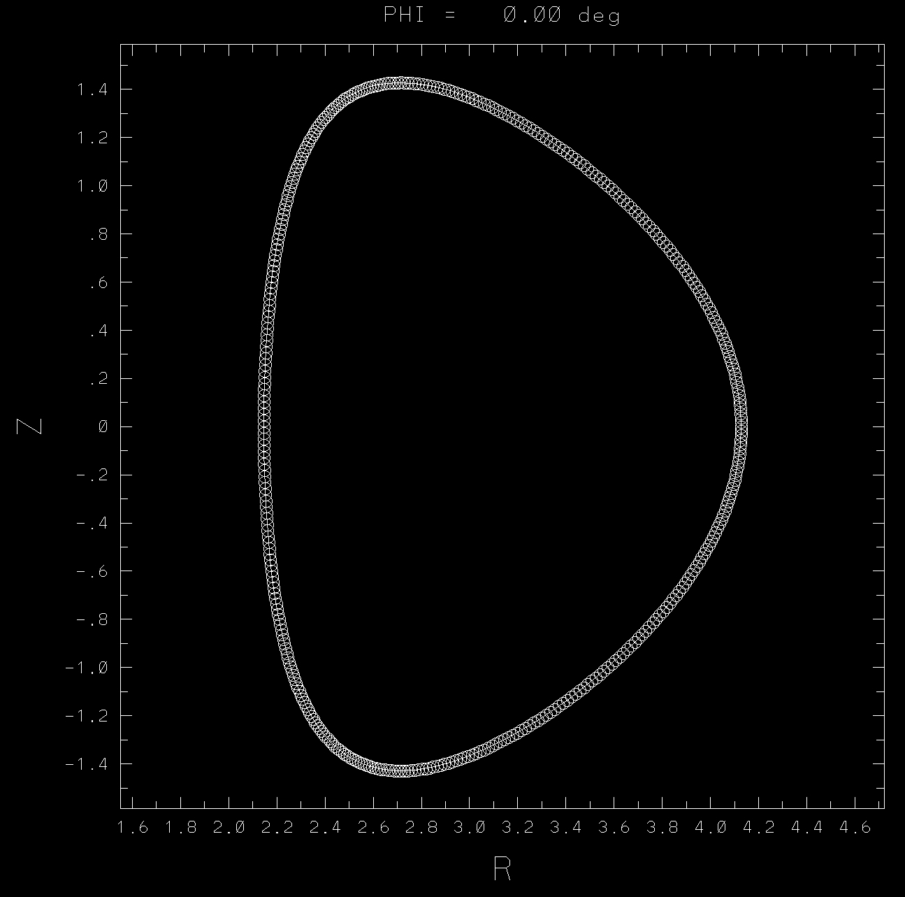
Visualization
The output of DESCUR code can be visualized with the DESCUR_PLOT code. This code produces contour plots of the Fourier Spectrum and a plot of the boundary based on the toroidal angle requested durring the execution of DESCUR.
Tutorials
Put links to tutorial pages here.