Code Name
The Princeton Iterative Equilibrium Solver (PIES) code calculates MHD equilibria for fusion devices with magnetic islands and stochastic regions.
Theory
The PIES (Reiman, A. and Greenside H. "Calculation of three-dimensional MHD equilibria with islands and stochastic regions." Comp. Phys. Comm., 43 (1986), Reiman, A. H. and Greenside, H. S. "Numerical solution of three-dimensional magnetic differential equations." Journal of Comp. Phys., 75 (1988), Greenside, H.S., Reiman, A. H., and Salas, A. "Convergence properties of a nonvariational 3D MHD equilibrium code." Journal of Comp. Phys., 81 (1989), Reiman, A. H. and Greenside, H. S. "Computation of ß three-dimensional equilibria with magnetic islands." Journal of Comp. Phys., 87 (1990)) code solves for MHD force balance using an iterative technique. This iterative technique can be summed up in three steps: > 1. The current perpendicular to the field lines is calculated from
> math \vec{j}_\perp = \frac{\vec{B}\times\nabla p}{B\^2} math
> 2. The parallel current is then solved on good flux surface (flattened in islands and stochastic regions) by:
> math \vec{B}\cdot\nabla\left(\frac{j_\parallel}{B}\right)=-\nabla\cdot\vec{j}_\perp math
> 3. The current is then used to solve for the magnetic field > math \nabla\times\vec{B} = \vec{j} math
The code uses two coordinate systems. The first is a background coordinates system which is similar to the VMEC coordinate system. Here the coordinates are Fourier decomposed in the poloidal and toroidal angle (using the kernel nv-mu, PIES coordinates), and discretized in the radial direction. The second coordinate system is magnetic, obtained by field-line following.
The PIES Coordinate systems
The PIES code uses both background and quasi-magnetic coordinate systems. The background coordinate grid is Fourier decomposed in the toroidal and poloidal directions and radially discritized. This coordinate system does not change from iteration to iteration and can be thought of as the grid on which the plasma moves. The background grid serves as the grid upon which the Poisson equation is solved for the field (Ampere's Law). The vacuum field is also stored on this grid. The quasi-magnetic coordinate system is determined by field line following. math \zeta=r cos \theta \eta=r sin \theta math This is the coordinate grid upon which the currents are calculated. This is done because quasi-magnetic coordinates are a natural coordinate system on which to calculate quantities such as current in the presence of islands and stochastic regions. In this coordinate system math \vec{B}=\nabla\Psi\times\nabla\theta+\iota\nabla\Phi\times\nabla\Psi+\vec{b} math where b/B is very small on good flux surfaces.
Field Line following
The PIES magnetic coordinate system is constructed from field line tracing. Tracing of the field lines is accomplished through integration of two ordinary differential equations math \frac{d\theta}{d\Phi}=\frac{\vec{B}\cdot\nabla\theta}{\vec{B}\cdot\nabla\Phi} math math \frac{d\rho}{d\Phi}=\frac{\vec{B}\cdot\nabla\rho}{\vec{B}\cdot\nabla\Phi} math Quantities are then Fourier transformed along field lines with a Gaussian window function applied. This allows analytic error estimates for the quantities which are not necessarily periodic.
Ampere's Law solvers
The PIES code employs two methods for solving for the magnetic field from the plasma currents. The primary way recognizes that Ampere's Law can be written as the solution to a three-dimensional Poisson solution. Here a field 'h' can be calculated from j math \nabla\times\vec{h}=\vec{j} math This field h does not follow the solenoidal constraint of the magnetic field (namely being a divergence free vector field). This allows for a divergence cleansing scheme to be employed. Here the magnetic field is written in terms of h and some scalar quantity u math \vec{B}=\vec{h}+\nabla u math The solenoidal constraint on the magnetic field then gives us a Poisson equation for u math \nabla\^2 u=-\nabla\cdot\vec{h} math An assumption of a fixed outer flux surface provides a Neumann boundary condition on u, namely math \left(\vec{h}+\nabla u\right)\cdot\nabla\Psi=\vec{B}\cdot\nabla\Psi=0. math
The secondary method for solving Ampere's law involves solving for the vector potential from the currents. Here the current gives rise to the vector potential and the vector potential gives rise to a divergence free magnetic field.
Compilation
The PIES code is maintained in a CVS repository. Once the code is check out into a sandbox the user must execute a setup script called makemake. Once makemake has been run the user should create a compilation directory. This is the directory in which the PIES source, objects, and executable will be compiled. The code is then compiled using gmake. At compilation time the user must provide gmake with the path to the compilation directory, and which machine the code will be compiled on. Durring the compilation process a series of macros are expanded in the code, along with conversion of the files from RATFOR Fortran to Fortran90.
Input Data Format
The PIES input file is a text file containing various name lists and data which sets up the coordinate system and initializes the fields. The PIES code was written to be a development environment so the name lists can have many variables. Only the basics of how to run the code are presented here. The first line of the input file is a string which indicates if the code should be restarted from
'begin'
&INPUT
  ITER2 = 5000   ! Max number of iterations
  CONVG = 1.000E-06   ! Convergence Criterion
  NUMLST = 2          ! Number of additional namelists
!-----  GRID Control Parameters  -----
  K = 70                              ! Number of radial grid surfaces
  M = 12                              ! Maximum number of poloidal modes
  N = 6                               ! Maximum number of toroidal modes
  MDA = 12                            ! Maximum number of poloidal modes for dealiasing
  NDA = 6                             ! Maximum number of toroidal modes for dealiasing
  MDSLCT = 1                          ! Mode selection matrix (0: Use all, 1: read matrix, 2: use m/2 n/2)
!-----  FIELD LINE FOLLOWING  -----
  NFOLMX = 90000                      ! Maximum number of periods for which field lines are followed
  FTPREC = 1.000E-05                  ! Relative accuracy with which Fourier amplitudes are determined
  FTFOL = 1.000E-05                   ! Tolerance for FFT for field line following
  LININT = 524288                     ! Number of points in Fourier Transforms (should equal a power of 2)
  LINTOL = 1.000E-07                  ! Tolerance in field line following
  DKLIM = 2.000E-03                   ! Maximum resolution in k space
  DEVPAR = 1.0                        ! Maximum deviation of field line (=devpar/k)
!-----  CONFIGURATION  -----
  NPER = 1.000                        ! Number of Field Periods
  RMAJ = 1.500                        ! Semi-major axis
  CYL = F                             ! Infinite Aspect ratio
  FREEB = T                           ! Free Boundary Run
  VMECF = 1                           ! Read VMEC Coordinates
  BSUBPI = -3.000                     ! B_phi on Axis
  SETBC = 1                           ! Boundary Condition (0: Flux Surface, B.n=0 1: Bad surface)
  ISLRES = 1.000                      ! Minimum island size (radial) to flatten pressure
  TOKCHK = 0                          ! Check for reasonable Tokamak Values
!-----  Rotational Transform Information  -----
  IOTAMX = 1.000                      ! Maximum Iota (rotational transform)
  IOTAMN = 0.200                      ! Minimum Iota
  RELIOT = 0.001                      ! Relative Error for iota solver (set to 0.0 for machine precision)
  ABSIOT = 0.001                      ! Absolute Error for iota solver (set to 0.0 for machine precision)
  MAXIOT = 100                        ! Maximum number of iterations in iota solver
!-----  PROFILE Parameters  -----
  IPRIMF = T                          ! Toroidal (T) or Poloidal (F) current specified
  ISPLN = 2                           ! Spline (p & dI/dpsi) profile (0: Off, 1: Spline wrt rho, 2: Spline wrt psi_norm, 3: use <J.B> wrt psi_norm)
  LP = 70                             ! Number of breakpoints for p spline
  BETA = 1.25663706143592E-06         ! Pressure scaling factor (4*pi*mu0, magnetic units)
  LJ = 70                             ! Number of breakpoints for I spline
  BETAI = 3.44147933418833E-07        ! Current scaling factor
  RTOKFK = 0.830                      ! The profile goes to zero at the kfth surface (rtokfk=kfth/k)
  LPINCH = 69                         ! All surfaces beyond this surface are considered bad
  ADJST = 0                           ! Adjust toroidal current profile to keep total current fixed
  IOTE = 3.14159                      ! Total current (I*mu0/2pi) to adjust profiles to match
!-----  Plots  -----
  PLTQLT = 0                          ! Plot quality (0: high, 1: medium, 2: low)
  AXDIAG = 0                          ! Plot Axis Finding Diagnostic
  AX1 = -0.1                          ! X-Minimum for axis diagnostic plots
  AX2 = 0.1                           ! X-Maximum for axis diagnostic plots
/
&PLTFLG
!-----  General Plotting Switches  -----
  PLTSF   = 1                         ! Use new plot flags
  PLTALF  = 0                         ! Plot All Modes (old way)
  IOTAF   = 1                         ! Unfiltered rotational transform (iota)
  QF      = 1                         ! Unfiltered safety factor (q)
  DELTAF  = 1                         ! Plots change in X, BPHI, BXY, and Iota
  DNTUP1F = 0                         ! JBUP (in hfldmn)
  DNTUP2F = 0                         ! JAUP (in psnrhs)
  DNTUP3F = 0                         ! JBUP (in newbup)
  RESDLF  = 0                         ! Plots residuals for each mode
  EDGEFL  = 0                         ! Plots plasma edge as function of iteration
  EDGF1   = 0                         ! Plots surfaces bounding islands (in polar plot)
  EDGF2   = 0                         ! Plots surfaces bounding islands (in rho-theta plot)
  EDGF3   = 0                         ! Plots sqrt of distance vs theta for islands.
  ISLPLT  = 0                         ! Plots island edges
  FREEBP  = 0                         ! Diagnostic plots for free boundary mode
!-----  Poincare Plotting Switches  -----
  POINCAF = 1                         ! Poincare in background coordinates
  POINCF  = 1                         ! Poincare plot in cartesian coordinates on last iteration only
  POINCM1 = 1                         ! Plot phi=0 plane in cartesian coordinates
  POINCM2 = 1                         ! Plot quarter and half filed period in cartesian coordiantes
  POINCMG = 1                         ! Surface control in Poincare plots (0: plot all, 1: plot to hitsrf, 2-4: see poincm routine)
  RPOINCF = 1                         ! Poincare in background coordinates (semi-polar plot, rho vs. theta)
  RPOINC_PLOT_RHO = 1                 ! Overplot on semi-polar plot (0: none, 1:, 2: )
  HUDSON_EDGES_PLT = 1                ! Overplot hudson separatrix
  WRITE_POINCARE_COORDINATES = 0      ! Output the real-space poincare data to files.
!-----  Coordinate/Jacobian Plotting  -----
  RHOMAGF = 0                         ! Plot rho and theta magnetic coordinates
  XPLTF   = 1                         ! r vs rho and theta vs theta_mag
  XIJF    = 0                         ! Plots of rr, xx, and yy on ij
  UFXF    = 0                         ! Unfiltered plots of X
  XMAGF   = 0                         ! Plot X(r) and Y(r) before and after call to pieces
  XMAGPEF = 0                         ! Plot or X(r) and Y(r) after pieces
  MODAMXF = 0                         ! Mode Amplitudes for X and Y after pieces
  RIJF    = 0                         ! Plot r and theta on ij
  DXF     = 0                         ! Plot gradients of cartesian coordinates (X,Y) as functions of magnetic coordinates
  RHOJAF  = 0                         ! Plot rho Jacobian (in parallel current calculation)
  BJACF   = 0                         ! Plot BPHI and rho Jacobian (in jacobs)
  DPSDNF  = 1                         ! D(PSI)/D(rho) in good regions (in parallel current calculation)
  DPSDNIF = 1                         ! D(PSI)/D(rho) interpolated (in parallel current calculation)
  IRREG_GRID_PLOT = 0                 ! Plot the irregular grid
!-----  Surface Plotting Switches  -----
  VESSELF = 0                         ! Add vessel data to real space plots (requires modification of vvsect subroutine)
  BACKF   = 1                         ! Background coordinate surfaces
  BGNDF   = 1                         ! Background coordinate grid
  MAGGNF  = 1                         ! Magnetic coordinate grid (before interpolation)
  MAGGNAF = 1                         ! Magnetic coordinate grid (after interpolation)
  MAGSNFF = 1                         ! Magnetic surfaces (after interpolation)
  RHOMAGF = 1                         ! Magnetic rho and theta coordiantes
!-----  Pressure Plotting Switches  -----
  DPDPSI_PLOT = 1                     ! Dp/Dpsi
  PMNF    = 1                         ! Pressure as a function of magnetic coordinates
  PMMNF   = 1                         ! PM in magnetic coordinate
  PMIJF   = 1                         ! PM on ij in magnetic coordinates
  PMIJBF  = 1                         ! PM on ij in background coordinates
  PRESSURE_CONTOUR_PLT = 1            ! Pressure contours in background coordinates
  DP1F    = 1                         ! Dp/Dr (in fjperp)
  DP23F   = 1                         ! Dp/Dtheta and Dp/Dzeta (in fjperp)
!----- Current Plotting Switches  -----
  MUMNF   = 1                         ! Parallel current in magnetic coordinates
  MUIJF   = 1                         ! Parallel current on ij in magnetic coordinates
  MUIJBF  = 1                         ! Parallel current on ij in background coordinates
  JJUPF   = 1                         ! Plot psi Jacobian (for local current density or plots JJUP)
  JPSJUP  = 1                         ! Plot psi Jacobian
  JPF     = 1                         ! Plot Jpup
  JJUPMF  = 1                         ! Plot jjup
  JJUPIJF = 1                         ! Plot jjup on ij
!-----  Magnetic Field  -----
  VMECBFP = 1                         ! Plot VMEC input field
  BUPFL   = 1                         ! Plot BUP
  BPHIF   = 0                         ! Plot B_PHI (in parallel current calculation)
  BPHIBF  = 0                         ! Plot unfiltered B_PHI
  MODBPF  = 1                         ! Plot magnitude of B
  BXBYFL  = 0                         ! Plot BX BY
  UBXBYF  = 0                         ! Plot unfiltered BX BY
/
&EXLSTA
!-----  General Options  -----
  BLEND_B = 0.99                      ! Blending factor (% of old solution to keep)
  UMINV = 5                           ! Curl inversion operator control (5: calculate pqqbtms, 6: read pqqbtms)
  NSAV = 50                           ! Save netCDF output ever NSAV iterations
  USE_VACFLD_KMAG = 0                 ! Use HINT vacuum field file (otherwise use coil field from Merkel code)
  CALCULATE_BVAC_ONCE = 1             ! Only calculated the vacuum field once
  STORVAC = 1                         ! Stores vacuum field in BVAC
  LOCAL_J = 1                         ! Use dp/dpsi to calculate current locally
  VIRTUAL_CASING = 1                  ! Use two pass virtual casing principle for boundary condition
  IFTMTH = 3                          ! Determines form of FFT (1: Hartley-libmath, 2: FFT-libsci, 3: fft-netlib, 4: fft-NAG-C06FPE)
  FBCF = 0                            ! Print out FBC array
  MDBSF = 0                           ! Print out surface quantities
  DEV_VMEC_F = 0                      ! Print out deviation from VMEC surfaces
  KERNBICHLER_WRITE = 0               ! Print out B and X in norm on final iteration (iter2)
  WRITE_EDGE_DATA = 0                 ! Print out plasma-vacuum interface modes on last iteration (if HUDSON_DIAGNOSTIC = 1)
  BOOTF = 0                           ! Calculate Bootstrap current (stellarator with no-loop voltage)
  ISDEFAULTISININ = 0                 ! Code should read the ISDEFAULT namelist
!-----  Field Line Following -----
  IAXBIS = 0                          ! Axis Root Finder (1: bisection and secant, iter =0 only; 2: bisection and secant for all iterations)
  NAXTOL = 0                          ! Set's field line following tolerance to foltol = lintol*10^(naxtol), for AXIS calculation
  LINTOLF = 1                         ! Do not reset LINTOL
  USE_LSODE = 0                       ! Use LSODE for field line following.
!-----  VMEC Related  -----
  VMECBF = 1                          ! Read VMEC B-Field (B^U,B^V) from input
  READ_BRHO = 1                       ! Read Radial VMEC B-Field (B^S from NMORPH) from input
  VMEC_IGNORE_SYM = 1                 ! Ignore VMEC Symmetry
  USE_POLY_FOR_CURRP_PRESS = 1        ! Read the AM and AC arrays from input file (note: ISPLN should be set to 2)
  BLOAT = 1                           ! Bloating factor for profiles (included for consistency with VMEC bloat factor)
  HIRSHF = 0                          ! Write out VMEC R,Z Fourier Arrays (background coordinates)
  DEV_VMEC_F = 0                      ! Write out deviation of field lines from background coordinates on final iteration (.dev file)
  REMOVE_CURRENT_IN_VACUUM_REGION = 2 ! Set the current to zero outside the last good flux surface.
!-----  STOCHASTIC Options -----
  MU_STOCHF = 0                       ! Stochastic current calculation (including rhobar)
  KSTOCH = 68                         ! Flatten profiles beyond this surface
  GRADFL = 1                          ! Gradual Flattening of pressure profiles in islands and stochastic regions
  ISLRE2 = 2.0                        ! Island size for complete flattening (radial grid units)
  LINEAR_INTERPOLATE_STINE_COORD = 1  ! Use linear interpolation in bad regions
  JDEV_CAL_FROM_DEV_IN_POLAR_COOR = 1 ! Jdev is found by deviation in polar coordinates.
  DEV_NORM = 1                        ! Calculate scale length for normalization of jdev
  ISMHMU = 1                          ! Switch to smooth mu by removing the resonant components
  ISMHMU_P = 0                        ! Smooths mu for cases with non-monotonic iota
  MOREMU = 1                          ! Use parallel current on surfaces adjacent to bad ones
  DEVRAT = -1                         ! (>0) Use DEVRAT to determine out of phase islands by local deviations.  (Do not use with HUDSON_EDGES)
  OUT_OF_PHASE = 0                    ! Treat out of phase islands
  ISLEDGF = 1                         ! Calls isledg to calculate island edges
  IBISEC = 10                         ! Number of bisections to use in island edge calculation
  BOOT_MODEL_F = 0                    ! Zero Current in islands
  HUDSON_DIAGNOSTIC = 0               ! Use Hudson diagnostic on last iteration (ITER2) to calculate island widths
  HUDSON_EDGES = 0                    ! Use Hudson diagnostic to determine edges of out of phase islands
  HUDSON_EDGES_IN_PHASE = 0           ! Use Hudson diagnostic to determine edges of in phase islands
  EDGDVF = 1                          ! Use edgedv rather than edge for calculating island edges
  JKLMF = 1                           ! Restore value of jklim from field line following if xiterzc fails
!-----  Grid Options -----
  IRREGULAR_GRID = 0                       ! Turn irregular grid on
  DKLIM_IRREG_GRID_INPUT = 2.0E-3          ! Minimum grid spacing for irregular radial grid
  USE_POLAR_COORD_TO_MAP = 1               ! Use polar coordinates to map background coordinates
  FLUX_QUADRATURE = 1                      ! Controls determination of toroidal flux (0: dpsdr, 1: dpdpsi, 2: psi)
  USE_INTERPOLATED_GRID = 1                ! On restart use interpolate background coordinates (best to set VMECF=0)
  ISMTHM = 1                               ! Smooth the quasi-magnetic coordinate by neglecting surfaces next to islands
  IRMVXM = 0                               ! Smooth the quasi-magnetic coordinate by removing the resonant components
  ISTNXM = 1                               ! Use Stineman interpolation on magnetic coordinates
  IMAPMG = 1                               ! Use vectorized version of magpmgf
  IDAGTR = 0                               ! Use trig transforms optimized for diagonal selection matrix
  SPIMTH = 2                               ! 1:  2: Use spectral inverse from fft of 1/quantity
  IWRTMG = 1                               ! Writes magnetic coordinates to 'magco.out' on last iteration.
  CHANGE_JKLIM_IF_OVERLAP_OF_MAG_COORD = 0 ! Set JKLIM=1 if coordinates overlap by value/k. (set to -1 to turn off)
!-----  Spline Options  -----
  USE_EZSPLINE_INTERP = 1             ! Use ezspline package for interpolation
  USE_EZSPLINE_IN_FBPH_AND_CRDINT = 1 ! Use ezspline package for FBPH and CRDINT
  USE_SPLINES_TO_INVERT_COORDINATES=1 ! Use splines to invert coordinates
  B_XSI_B_ETA_TEST = 1                ! Test splining routine
  USE_SPLINE_DER_FOR_PRESS = 0        ! Calculate dp/dr (dp/dpsi) from Splines directly
!-----  Coil Related -----
  FAC_NESCOIL = -1.0000E-7            ! Scaling factor for current in coils
  NW = 0                              ! Number of coil filament nodes
  DYNAMICAL_HEALING = 0               ! Conduct coil healing of islands
  DYNAMICAL_HEALING_RESTART_ITER = 0  ! Restart iteration for a healing run from free boundary
  WRITE_BDOTN = 0                     ! Write B dot N on last surface (fort.26)
  SETBC_OVERRIDE2 = 0                 ! Allows restart from a fixed boundary run to free boundary for one step coil healing
!-----  Error handling Options -----
  ISTOP = 0                                  ! Switch to stop the code at various points
  CHECK_POINT_FLAG = 0                       ! Writes to ~/Tmp in case machine crashes
!-----  Chebyshev Parameters -----
  CHEBYF = 0                          ! Use Chebyshev Blending
  NCYC = 0                            ! Length of Chebyshev cycle to use
/
Execution
The code is executed by passing it the name of an input file as a command line argument to the code. For example to run PIES for a case specified by test.in the command would look like:
> ~/bin/pies test
If run in free boundary the PIES code will also require a coil definition file coil_data in the same directory as the input file. If the code is to be run as a restart then an netCDF file will also be required. For example, if you wish to run test.in as a restart you'll also need a test_old.nc file.
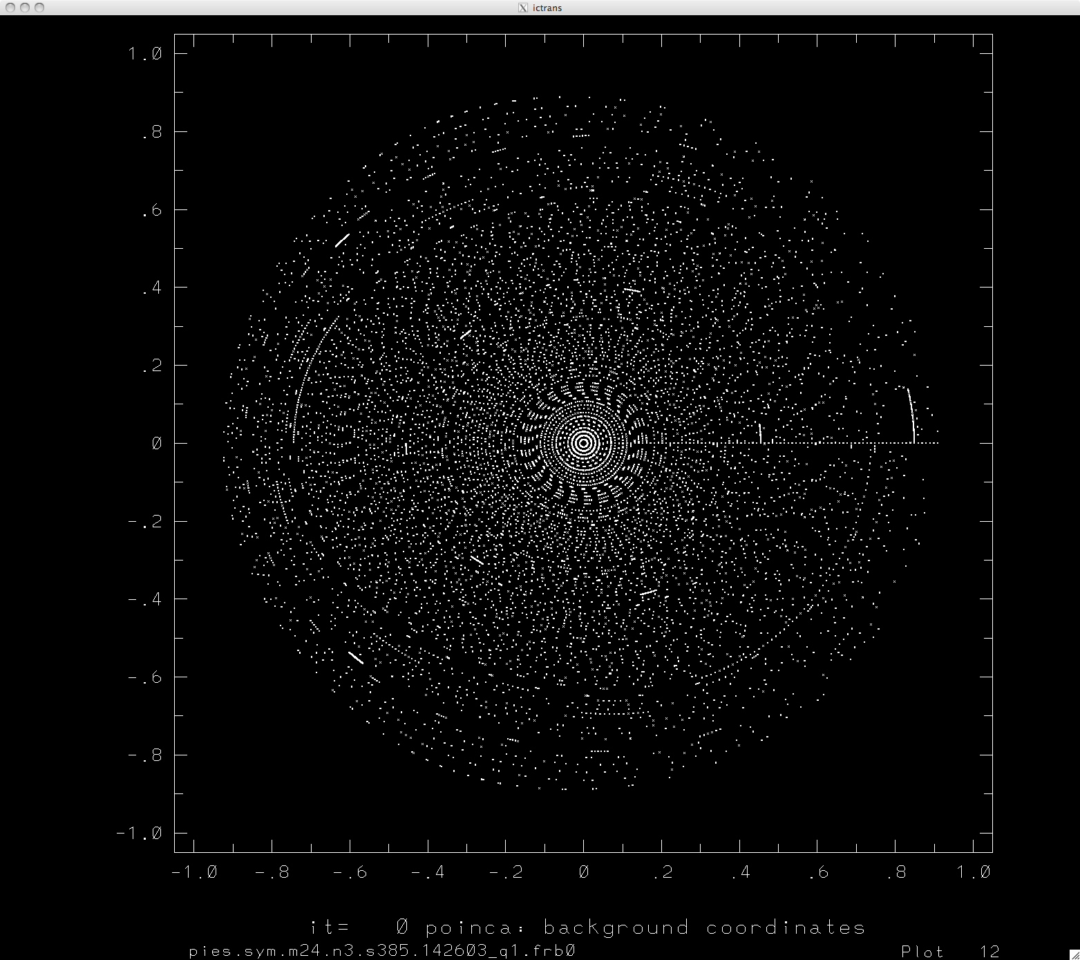
The PIES code can be run as a single iteration field line tracer. To do this the POINCMG should be set in the PLTFLG name list (along with WRITE_POINCARE_COORDINATES) to the desired value. The ISTOP variable should be set to 37 in the EXLSTA name list. The ITER2 variable (in the INPUT name list) should be set to 1 or one iteration larger than is stored in the restart file. The code will then produce the Poincaré plots and exit.
Output Data Format
The PIES code produces 3 main output files. The first is a '.out' file which contains more verbose output for the run than that printed to the screen durring execution. The '.gmeta' file contains the various plots that the code produces durring execution. It is an NCAR Command Language (NCL) Computer Graphics Metafile. It can be read with the ctrans (or ictrans) applications. The '.toc' file contains a list of the plots in the '.gmeta' file. The code also outputs it's data to a netCDF file by the name 'test_save.nc'. Also the NSAVE parameter in the EXLSTA input namelist can be set so that every NSAVE iterations the netCDF file copied to an file with the iteration number appended as a suffix. The netCDF file contains various variables describing the equilibria. Of particular interest are the variables 'relbup_old' which contains the contravariant Fourier components (B_rho, B_theta, B_phi) of the magnetic field, and 'x' which contains the Fourier components of the background coordinates.
Visualization
The PIES code preforms it's own data visualization. The '.gmeta' file contains the plots and can be view with the ctrans (or ictrans) applications. The '.toc' file contains a list of the plots in the '.gmeta' file. The plotting of the code is controlled by the PLTFLG input namelist. A common request for a user is to create a real-space Poincaré plot from an output. This is usually only done on the final iteration as it does take some time to render in the code and is not necessary part of the codes computation. See the tutorials below. Also note that the user may add to the real space plots through the vvsect routine.
The matlabVMEC routine can visualize quantities on the background coordinates from a PIES netCDF file. In order to do this the user must first read the PIES netCDF file in MATLAB using the read_pies_netcdf function. The user then passes the pies data structure to VMECplot and the relevant quantities are plotted.
Tutorials
Put links to tutorial pages here.