VMEC

The code uses a variational method to find a minimum in the total energy of the system. The code assumes that quantities may be Fourier expanded in terms of the poloidal and toroidal coordinates. This produces a parabolic set of equations (with second-order spatial derivatives in the radial coordinate, rho), which are converted to hyperbolic form through a Richardson scheme. The VMEC code is able to rapidly solve for MHD equilibrium configurations in magnetically confined fusion devices.

Theory

VMEC coordinates (*The toroidal angle used in VMEC is in the counter-clockwise direction)

The VMEC code seeks to solve a set of MHD force balance equations in a toroidal domain:

\(\vec{F}=-\vec{j}\times\vec{B}+\vec{\nabla}p=0,\)

\(\vec{\nabla}\times\vec{B}=\mu_o\vec{j},\)

\(\vec{\nabla}\cdot\vec{B}=0.\)

Combining these equations the total plasma potential energy can be written

\(W=\int\left(\frac{\|\vec{B}\|^2}{2\mu_o}+\frac{p}{\gamma-1}\right)d^3x.\)

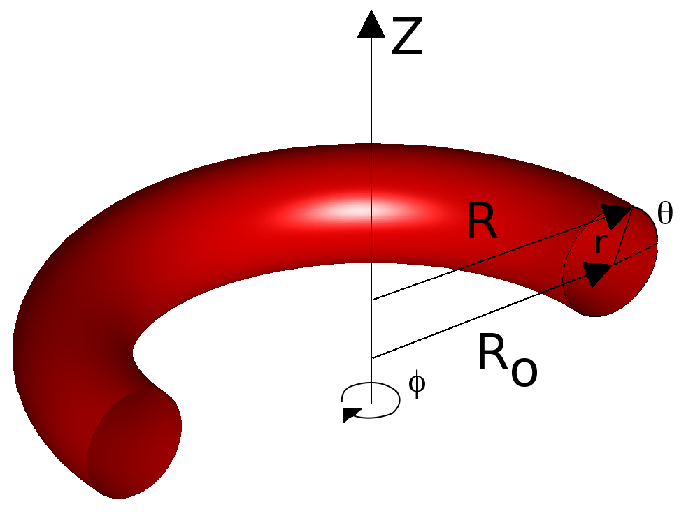
The scalar invariance of the potential energy allows it’s computation directly in flux coordinates. The relevant toroidal-cylindrical and flux coordinates are shown in Figure 1.

The flux and mass of the system must be conserved. The conservation of flux is achieved through a contravariant formulation of the magnetic field

\(\vec{B}\cdot\vec{\nabla}p=0\)

\(\vec{\nabla}\cdot\vec{B}=0\)

\(\longrightarrow\)

\(\vec{B} = \vec{\nabla}\zeta\times\vec{\nabla}\chi+\vec{\nabla}\Phi\times\vec{\nabla}\theta^*\)

\(= B^\theta \hat{e}_\theta + B^\zeta\hat{e}_\zeta\)

where \(\theta^*=\theta+\lambda\left(\rho,\theta,\zeta\right)\), and \(\lambda\) straightens the magnetic field lines. Adiabatic conservation of mass flux may then be achieved through

\(p\left(\rho\right)=\frac{M\left(\rho\right)}{\left[\int\int d\theta d\zeta \| \sqrt{g} \|\right]^\gamma} \qquad \sqrt{g}=\frac{1}{\vec{\nabla}\rho\cdot\vec{\theta}\times\vec{\nabla}\zeta}\)

where M is our mass function and g is the metric for the flux coordinates. This allows the total potential energy to be written as

\(W=\int\frac{\|\vec{B}\|^2}{2\mu_o}\|\sqrt{g}\|d\rho d\theta d\zeta + \int_0^1 \frac{M\left(\rho\right)}{\left(\gamma-1\right)\left[\int\int d\theta d\zeta \|\sqrt{g}\|\right]^{1-\gamma}}d\rho.\)

The magnitude of the magnetic field is defined as:

\(\|\vec{B}\|^2\equiv B^iB_i=\left(B^\theta\right)^2g_{\theta\theta}+2B^\theta B^\zeta g_{\theta\zeta}+\left(B^\zeta\right)^2g_{\zeta\zeta}.\)

The limits of the second integral indicate that we’ve normalized our radial magnetic coordinate to the dimensions of our toroidal cross section.

A variation in the potential energy is now preformed. The resulting equation may be written

\(\frac{dW}{d\beta}=\int\left[-\left(\frac{\|\vec{B}\|}{2\mu_o}+p\right)\frac{\partial \sqrt{g}}{\partial\beta}+\frac{1}{\mu_o\sqrt{g}}\left(b_R\frac{\partial b_R}{\partial \beta}+R^2b_\phi\frac{\partial b_\phi}{\partial \beta}+b_Z\frac{\partial b_Z}{\partial \beta}+Rb^2_\phi\frac{\partial R}{\partial \beta}\right)\right]d^3\alpha,\)

where a variational parameter (Beta) has been used instead of the canonical time (t). The toroidal-cylindrical domain considered here is defined by x=(R,phi,Z). Utilizing the coordinate transformation between the toroidal-cylindrical and magnetic coordinate domains we may then rewrite the variation in potential energy:

\(\frac{dW}{d\beta}=-\int F_i\frac{\partial x_i}{\partial \beta}d^3\alpha -\int F_\lambda \frac{\partial \lambda}{\partial \beta}d^3\alpha -\int_{\rho=1}\|\sqrt{g}\|\frac{\partial \rho}{\partial x_i}\left(\frac{\|\vec{B}\|^2}{2\mu_o}+p\right)\frac{\partial x_i}{\partial \beta}d\theta d\zeta.\)

Here, the MHD force components are \(\left(F_1,F_2,F_3\right)=\left(F_R,F_\phi,F_Z\right)\).

\(F_R=-\frac{\partial}{\partial \rho}\left[\|\sqrt{g}\|\frac{\partial\rho}{\partial R}\left(\frac{\|\vec{B}\|^2}{2\mu_o}+p\right)\right]-\frac{\partial}{\partial \theta}\left[\|\sqrt{g}\|\frac{\partial\theta}{\partial R}\left(\frac{\|\vec{B}\|^2}{2\mu_o}+p\right)\right]\)

\(-\frac{\partial}{\partial \zeta}\left[\|\sqrt{g}\|\frac{\partial\zeta}{\partial R}\left(\frac{\|\vec{B}\|^2}{2\mu_o}+p\right)\right]+\mu^{-1}_o\|\sqrt{g}\|\vec{\nabla}\cdot\left[\left(\vec{B}\cdot\vec{\nabla}R\right)\vec{B}\right]\)

\(+\frac{\sqrt{g}}{R}\left[\frac{\|\vec{B}\|^2}{2\mu_o}+p-\frac{R^2\left(\vec{B}\cdot\vec{\nabla}\phi\right)^2}{\mu_o}\right]\)

\(F_\phi=-\frac{\partial}{\partial \rho}\left[\|\sqrt{g}\|\frac{\partial\rho}{\partial \phi}\left(\frac{\|\vec{B}\|^2}{2\mu_o}+p\right)\right]-\frac{\partial}{\partial \theta}\left[\|\sqrt{g}\|\frac{\partial\theta}{\partial \phi}\left(\frac{\|\vec{B}\|^2}{2\mu_o}+p\right)\right]\)

\(-\frac{\partial}{\partial \zeta}\left[\|\sqrt{g}\|\frac{\partial\zeta}{\partial \phi}\left(\frac{\|\vec{B}\|^2}{2\mu_o}+p\right)\right]+\mu^{-1}_o\|\sqrt{g}\|\vec{\nabla}\cdot\left[\left(R^2\vec{B}\cdot\vec{\nabla}\phi\right)\vec{B}\right]\)

\(F_Z=-\frac{\partial}{\partial \rho}\left[\|\sqrt{g}\|\frac{\partial\rho}{\partial Z}\left(\frac{\|\vec{B}\|^2}{2\mu_o}+p\right)\right]-\frac{\partial}{\partial \theta}\left[\|\sqrt{g}\|\frac{\partial\theta}{\partial Z}\left(\frac{\|\vec{B}\|^2}{2\mu_o}+p\right)\right]\)

\(-\frac{\partial}{\partial \zeta}\left[\|\sqrt{g}\|\frac{\partial\zeta}{\partial Z}\left(\frac{\|\vec{B}\|^2}{2\mu_o}+p\right)\right]+\mu^{-1}_o\|\sqrt{g}\|\vec{\nabla}\cdot\left[\left(\vec{B}\cdot\vec{\nabla}Z\right)\vec{B}\right].\)

This defines our system of equations. This system is subsequently simplified through a spectral decomposition in the angle variables and furthermore through the implementation of a steepest-descent method for solving for the minimum in potential energy.

The inverse mapping (\(R,\lambda,Z\) in terms of the flux coordinates \(\rho,\theta,\zeta\)) can be expressed as:

\(R=R_o\left(\rho\right) + f_R \left(\rho,\theta,\zeta\right),\)

\(Z=Z_o\left(\rho\right) + f_Z \left(\rho,\theta,\zeta\right).\)

A Fourier expansion in terms of theta and zeta may be conducted giving

\(x_j=\sum_{m,n}X_j^{mn}\left(\rho\right)\exp\left[i\left(m\theta-n\zeta\right)\right]\)

where \((x_1, x_2, x_3)=(R, \lambda, Z)\). The variation of the total potential energy then becomes

\(\frac{dW}{d\beta}=-\int\left(F_j^{mn}\right)^* \frac{\partial X_j^{mn}}{\partial \beta}dV,\)

\(F_j^{mn}=\frac{1}{\partial V / \partial \rho}\int\int F_j\exp\left[-i\left(m\theta-n\zeta\right)\right] d\theta d\zeta.\)

Having simplified the equation through a Fourier decomposition we now see that the net Force in the system will be composed of second order operators in rho. A minimum in potential energy is now sought.

The method of steepest descent is used to progress towards a minimum in potential energy. This path is given by

\(\frac{\partial X_j^{mn}}{\partial \beta}=F_j^{mn}.\)

It is now assumed that the variational parameter beta can be taken to be the canonical time t. This equation is parabolic in nature. A second-order Richardson scheme may be applied to the derivative over the variational parameter to reduce this equation to a hyperbolic form and increase the rate of convergence. This equation then becomes

\(\frac{\partial^2 X_j^{mn}}{\partial \beta^2}+\frac{1}{\tau}\frac{\partial X_j^{mn}}{\partial \beta}=F_j^{mn}\)

where the optimum frequency is given by

\(\frac{1}{\tau_{op}}=-\frac{d}{d\beta}\left(\int \|F\|^2dV\right).\)

The spectral nature of the VMEC code coupled with the toroidal geometry of magnetic fusion devices reduces the number of boundaries to two along the rho dimension. The first is located at the origin (rho=0). Here three general constraints on the behavior of the magnetic field at the origin must be maintained. At the outer boundary (rho=1) two situations may exist: a fixed boundary and a free boundary. The former case is simply implemented through specification of the boundary Fourier amplitudes (\(X_j^{mn}\)). In the latter case, energy principles must be incorporated into the variational principle.

The magnetic field must be well behaved at the inner boundary. The magnetic axis must not have a poloidal dependence (theta). This implies that that all the Fourier coefficients (\(X_j^{mn}\)) must vanish at the origin for m≠0. The net force in the system is a second order operator in rho. This implies that at the origin, which has mirror symmetry, the Fourier coefficients must also be second order in rho. In terms of the Fourier coefficients (\({X_1^{0n}}' = {X_3^{0n}}'=0\), here the prime indicates a derivative with respect to rho. The final constraint is on the lambda coordinate. At the origin we require the poloidal derivative of the toroidal coordinate to vanish. Again in the nomenclature of the Fourier coefficients, it is written

\(\partial X_2^{0m}/\partial \theta=0.\)

It is also important to mention that the toroidal coordinate must be periodic thus it’s m=0,n=0 coefficient must vanish everywhere (\(X_2^{00}=0\)). This completes the boundary specification of the magnetic field at the origin.

The boundary conditions for a fixed outer boundary (rho=1) are implemented through specification of the Fourier coefficients. The shape of the flux surface thus prescribes the radial \(X_1^{mn}\) and vertical \(X_3^{mn}\) coordinate coefficients. The poloidal force components contain no radial derivatives. This implies that no boundary specification is required for \(X_2^{mn}\).

The VMEC code treats the ‘free’ outer boundary condition through inclusion of a ‘vacuum’ magnetic field. The MAKEGRID code is used to produce an ‘mgrid’ file. This file contains the vacuum field on an R-Z grid for a series of toroidal angles for a given coil set. The vacuum field can be decomposed into two parts

\(\vec{B_V}=\vec{B_0}+\nabla\Phi.\)

Here the first part is attributed to the plasma currents and coil configuration, the second part is a single valued potential. This potential is required in order to satisfy the following condition

\(\vec{B_V} \cdot \hat{n} = 0,\)

the flux surface constraint. At the vacuum-plasma interface the total pressure must be continuous and the normal component of the vacuum field must vanish. This field is incorporated into the total potential energy and a variation is conducted. This produces a descent equation for the vacuum potential

\(\frac{\partial \nu}{\partial \beta}=F_\nu\equiv-\vec{\nabla}\cdot\vec{B_\nu}=\nabla^2\nu.\)

The free boundary condition requires the calculation of the initial vacuum magnetic field from data involving the coil configuration. The MAKEGRID code is used to produce an ‘mgrid’ file. This file contains the vacuum field on an R-Z grid for a series of toroidal angles.

Compilation

VMEC is a component of the STELLOPT suite of codes. It is contained within the ‘stellopt.zip’ file. Compilation of the STELLOPT suite is discussed on the STELLOPT Compilation Page.

Input Data Format

The VMEC input file has the name ‘input.name’ where ‘name’ is a descriptive name of the user’s choosing. This input file is a Fortran namelist file which specifies how the code is to be run. A full listing of variable can be found in the input variable namelist page. The input file in general looks like:

&INDATA
LFREEB = F
MGRID_FILE = "none"
DELT = 0.9
NFP = 7
NCURR = 0
MPOL = 9
NTOR = 6
NZETA = 18
NITER = 10000
NSTEP = 200
NVACSKIP = 6
GAMMA = 0.000000E+00
PHIEDGE = 1.13E-01
CURTOR = 0.0
NS_ARRAY =     9      49
FTOL_ARRAY = 1.00e-6   1.e-11
AM =   1.e4    -1.e4    9*0.
AI =    6.90    0.0      0.0    3.90   0.0    0.0    6.90    0.0    0.0    6.90
0.0
AC =   11*0.
RAXIS =   2.88    0.04
ZAXIS =   0.00   -0.04
RBC(0,0) =   2.90     ZBS(0,0) =   0.00
RBC(0,1) =   1.00     ZBS(0,1) =   1.00
RBC(1,1) =  -0.21     ZBS(1,1) =   0.21
RBC(1,4) =  -0.01     ZBS(1,4) =   0.01
RBC(1,6) =  -0.01     ZBS(1,6) =  -0.01
/

The first line simply defines the Fortran namelist and the last line ends it. The ‘LFREEB’ is a boolean value which specifies if the code should be run in free boundary mode. If ‘LFREEB’ is set to ‘T’ then the next variable ‘MGRID_FILE’ must specify the name of an mgrid file created by the xgrid package. This file contains information regarding the fields created by the various field coils. If ‘LFREEB’ is set to ‘F’ then ‘MGRID_FILE’ is ignored and may be omitted. The ‘DELT’ parameter determines the amount of blending from previous iterations (value from 0.0 to 1.0). The ‘NFP’ variable specifies the number of field periods in the toroidal direction (number of times the plasma cross-section repeats itself). The ‘NCURR’ variable specifies that the rotational transform (NCURR=0, iota) or the toroidal current (NCURR=1) is specified at the boundary. The ‘MPOL’ variable specifies the maximum poloidal mode number for the run. The ‘NTOR’ variable specifies the minimum and maximum toroidal mode number for the run. The ‘NZETA’ variable specifies the number of planes on which the mgrid file has calculated the magnetic field. The ‘NITER’ variable specifies the maximum number of iterations for the VMEC code. Note that if this number is exceeded VMEC will continue to run for double this number to see if convergence can be met. The ‘NSTEP’ variable determines how often the code should output diagnostics to the screen and ‘threed1’ file. The ‘NVACSKIP’ variable is used for a free boundary run to indicate how often to update the vacuum field solution. The ‘GAMMA’ variable is used to set the adiabatic (compressional) index. Note that for GAMMA=0.0 the code assumes it is being supplied a pressure not a mass. The ‘PHIEDGE’ variable specifies the total enclosed toroidal flux for a fixed boundary run. For a free boundary run, this variable limits the radius of the plasma. The ‘CURTOR’ variable specifies the scaling for the toroidal current in Amps.

The ‘NS_ARRAY’ and ‘FTOL_ARRAY’ specify the radial grid refinement that the code uses. In general the code iterates on a given radial grid. Once a specified tolerance is met, the code uses a more refined grid and restarts it’s iterative cycle for a new tolerance. The ‘NS_ARRAY’ is an array of integers specifying the number of radial grid points for each cycle of the code. The ‘FTOL_ARRAY’ variable specifies the tolerance for a given radial grid discretization. These arrays should have the same number of elements. In this way the user control the gird refinement of the code.

The input profiles (mass/pressure, rotational transform, and current) for the code are described in terms of a 10th order polynomial in the radial grid. The user must thus specify the 11 coefficients for the polynomial in input file. The ‘AM’ array specifies the coefficients for the mass (pressure) polynomial. The ‘AI’ array specifies the coefficients for the rotational transform (iota) polynomial (used if NCURR=0). The ‘AC’ array specifies the coefficients for the toroidal current polynomial (used if NCURR=1). In order to change the specification to a form other than a polynomial in the radial direction, the source code for the profile specifications must be changed. The ‘pcurr.f’, ‘piota.f’, and ‘pmass.f’ files in the ‘vsource’ directory specify these profile functions.

The code requires a guess for the initial magnetic axis. The position of this axis is specified in the ‘RAXIS’ and ‘ZAXIS’ variables. The axis is specified by a space curve in terms of Fourier coefficients in the toroidal angle. The ‘RAXIS’ and ‘ZAXIS’ variables contain the Fourier coefficients describing this space curve. This is only an initial guess.

The boundary coefficients for the plasma are stored in the ‘RBC’, ‘RBS’, ‘ZBC’, and ‘ZBS’ variables. These are Fourier coefficients describing the outer most flux surface over one field period. For a fixed boundary run, these values prescribe the shape of the outer most flux surface. For the free boundary run, they prescribe an initial condition for the shape of the plasma. For up-down symmetric (stellarator symmetric) plasmas, only the ‘RBC’ and ‘ZBS’ coefficients need be specified. The variables names indicate if they reference radial (R) or vertical (Z) coordinates. The second character (B) specifies them as the boundary coefficients. The third letter specifies sine (S) or cosine (C) transformations. NOTE: The definition of the boundary also defines the sign of the poloidal and toroidal angles. For example, the choice of negative ZBS(0,1) implies the field will rotate in the clockwise direction when viewed in cylindrical coordinates. A negative value of iota is generally a good indicator that your boundary definition needs to be flipped.

It is worthwhile to note that the array indices in VMEC use toroidal angle precedence so the first index of the arrays is over the toroidal mode indices while the second is over the poloidal indices. Also remember that the toroidal angle must be multiplied by the number of field periods to plot the entire torus. This implies that ‘NTOR’ actually corresponds to NTOR x NFP modes over the entire torus.

Execution

To run VMEC with a given input file simply pass the suffix of the file to VMEC like so (input file named input.test):

yourmachine:0005> ~/bin/xvmec2000 test >& log.test &

Here we’ve redirected screen output (trapping error messages) to ‘log.test’ and put the process in the background.

Output Data Format

The VMEC code outputs some runtime and diagnostic data to the screen along with the creation of four files (jxbout, mercier, threed1, and wout). The data output to the screen is also indicated (in greater detail) in the threed1 file. It is suggested that the user redirect the output of the run to a log file. The wout file is a text file containing data from plotting of the final configuration. Details of reading the ‘wout’ file can be found in LIBSTELL/Sources//Modules/read_wout_mod.f90. If ‘LDIAGNO’ was set to true in the input namelist, a ‘diagno_in’ file will be created. This file contains information regarding the outer flux surface and currents for the DIAGNO routine (which calculate the field at a point for magnetic reconstruction).

Visualization

The datafiles output by VMEC are text files which explain the quantities they contain, the exception being the ‘wout’ file. This file contains a reduced form of the Fourier coefficients for various quantities, along with radial profiles of specific quantities. This file can be in text or netCDF format. The user is encourage to examine the files in the matlabVMEC package to better understand how to handle these quantities. In general, VMEC stores the R and Z data in the variables ‘rmnc’ and ‘zmns’. These variables are two dimensional. One dimension indexes the radial surface the other is a vectorization over the poloidal and toroidal modes. The ‘xn’ and ‘xm’ variables store the m and n information for a given index. It is important to note that VMEC calculates values over one field period, thus for a full torus one must multiply the toroidal mode number (n) by the number of field periods for a given machine. Strumberger provides an explanation of how to map the VMEC contravariant vectors to cylindrical space. A few packages exist to ease the user into plotting the VMEC data. A discussion of toroidal coordinate systems can be found Toroidal Coordinate. A FORTRAN library for manipulation of toroidal equilibria AJAX does exist and is distributed as part of the LIBSTELL package.

MATLAB: A series of utilities for reading and plotting VMEC and STELLOPT data can be found at the matlabVMEC Github repo. (https://github.com/lazersos/matlabVMEC)

IDL: ECHIDNA, provides a GUI for execution and visualization of VMEC via IDL.

Python: PySTEL is also available in the repository.

STELLOPT

References

- VMEC input variables on Doxygen
- Hirshman, S.P. and Whitson, J.C. "Steepest-descent moment method for three-dimensional magnetohydrodynamic equilibria." Phys. Fluids 26, 3353 (1983)
- Hirshman, S.P. and Meier, H.K. "Optimized Fourier representations for three-dimensional magnetic surfaces." Phys. Fluids 28, 1387 (1985)
- Hirshman, S.P. and Lee D.K. "Momcon: A spectral code for obtaining three-dimensional magnetohydrodynamic equilibria." Comp. Phys. Comm. 39, 161 (1986)
- Hirshman, S.P., van Rij, W.I., and Merkel P. "Three-dimensional free boundary calculations using a spectral green’s function method." Comp. Phys. Comm. 43, 143 (1986)
- Hirshman, S.P. and Betancourt O. "Preconditioned descent algorithm for rapid calculations of magnetohydrodynamic equilibria." J. Comp. Phys. 96, 99 (1991)
- E. Strumberger, S. Günter, P. Merkel, E. Schwarz, C. Tichmann and H.-P. Zehrfeld "Numerical computation of magnetic fields of two- and three-dimensional equilibria with net toroidal current." Nuclear Fusion 42, 7 (2002)
- S.E. Attenberger, W. A. Houlberg and S.P Hirshman. "Some practical considerations involving spectral representations of 3D plasma equilibria." J. Comp. Phys. 72, 435 (1987)
- S.A. Lazerson, J. Loizu, S.P. Hirshman, and S.R. Hudson "Verification of the ideal magnetohydrodynamic response at rational surfaces in the VMEC code." Phys. Plasmas 23, 012507 (2016)