Grids
Documentation/ProgrammerGuide/Grids
Every Domain in the Mesh is composed of at least one Grid. For serial calculations on a single processor, there is only one Grid per Domain. For MPI parallel calculations, there may be one or more Grids per Domain, depending on the decomposition.
Indexing Cells on a Single Grid
The Grids contain cells in a regular mesh in which the discretized solution is stored and updated. The cells are referenced according
to integer indices i,j,k.
As an example, consider a serial calculation without SMR. In this case there is only one root Domain, which contains one Grid.
The figure below shows the integer coordinate system which is used to label cells on this single Grid, and the relationship between the
physical coordinates (x1,x2) and the integer indices.
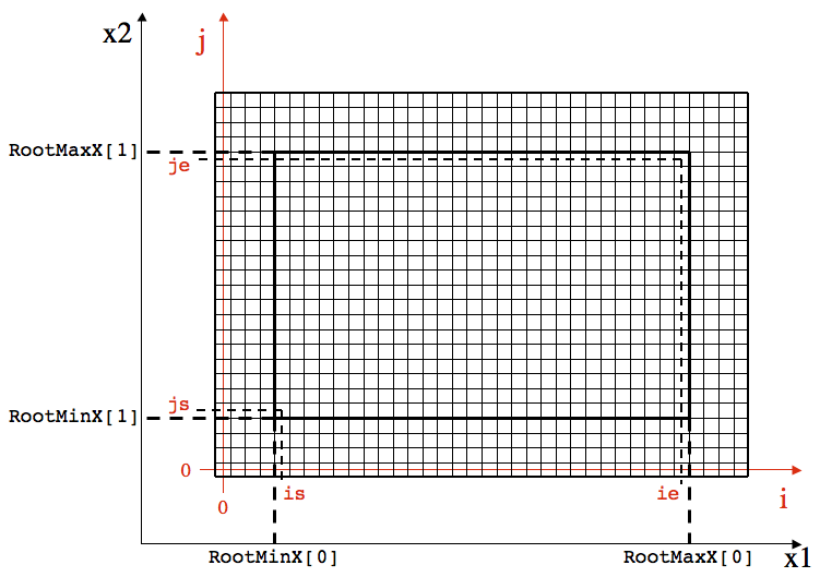
The bold black line denotes the volume of physical space covered by the root Domain (which is the same as the single Grid in this example).
This region spans RootMinX[i] ≤ x[i] ≤ RootMaxX[i], for i=0,1.
Note that the region covered with Grid cells extends beyond the physical region associated with
the root Domain. The extra cells beyond the edge of the Domain are called ghost zones, and they are used to apply boundary conditions to the
solution.
To avoid indexing arrays with negative integers, the first ghost zone in the lower-left in each dimension has index zero. The cell-centered
location of the first active cell on the Grid has indices (is,js,ks) in the (i,j,k) directions. Generally, is=nghost, where
nghost is the number of ghost cells, and similarly for js and ks. The last active cell has
indices (ie,je,ke) in the (i,j,k) directions. Generally, ie=Nx[0]+nghost-1, where Nx[0] is the total number of actively updated
cells in the x1-direction, similarly for je and ke.
The integer indices of Grid cells refer to the locations of cell centers, not cell edges. Thus, the transformation between the physical
(x1,x2,x3) coordinates and the integer (i,j,k) indices is given by (in C code).
x1 = RootMinX[0] + ((Real)(i - is) + 0.5)*dx1;
x2 = RootMinX[1] + ((Real)(j - js) + 0.5)*dx2;
x3 = RootMinX[2] + ((Real)(k - ks) + 0.5)*dx3;
where dx1,dx2,dx3 are the physical size of individual Grid cells, which must be a constant (the same for all cells on all Grids
at the same level).
In general, the transformation is somewhat more complicated, because the Grid may be only part of a Domain that is embedded in the
root Domain (remember, the above example is for a single Grid which covers the entire root Domain). The more general case
is described below.
Indexing Cells on Grids: the General Case
The figure below diagrams how the positions of Grid cells are related to the physical coordinates in the more general case of a level=1 Domain embedded in a root Domain. Any other configuration of levels and Domains can be represented in a similar fashion.
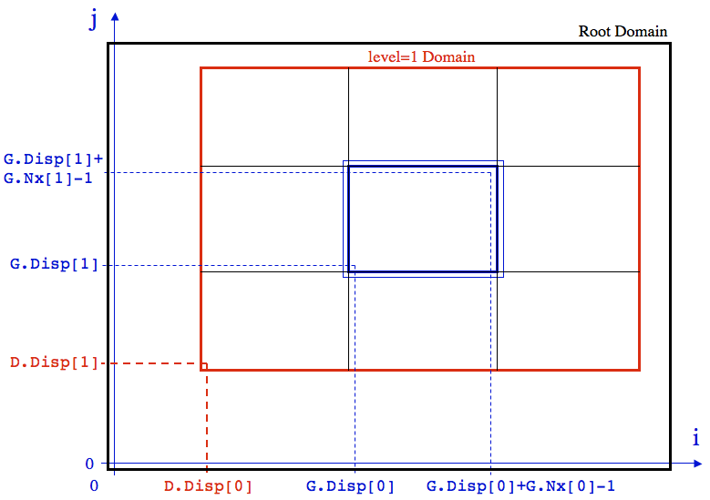
As in the example above, the bold black line denotes the volume of physical space covered by the root Domain. The bold red line denotes the volume of physical space covered by the level=1 Domain. Finally, the bold blue line denotes the volume of physical space covered by the actively updated cells on a particular Grid on the level=1 Domain. The light blue line slightly beyond this volume is the region covered by all cells in this Grid, including the ghost zones. Note that the ghost zones overlap with the volumes covered by neighboring Grids; in this case values in the ghost zones would be set via MPI calls which pass data from those other Grids.
The physical coordinate system x1-x2 is not shown in this figure to keep it simpler, however, as shown in the second figure in
the section on Domains, the edges of the root Domain are RootMinX[i]
and RootMaxX[i] for each direction i,
while the edges of the level=1 Domain are located at MinX[i] and MaxX[i] for each direction i.
The location of the first, actively updated Grid cell (labeled by (is,js) on this Grid) relative to the origin
of an integer coordinate system that covers the entire computational volume (root Domain) is given by an integer displacement
G.Disp[0]. The location of the last (in each direction), actively updated Grid cell (labeled by (ie,je)
on this Grid) is given by G.Disp[i]+G.Nx[i]-1, where G.Nx[i] is the number of actively-updated cells on this Grid in each direction.
The origin of the integer coordinate system that labels Grid cells on this level corresponds to the center of the first actively
updated cell on the root Domain.
The prefix G. is used to schematically represent a structure associated with the Grid that stores these displacements.
The actual Grid structure used has a different name. However, this schematic name is needed to
distinguish between the integer displacement of the first, actively-updated cell in each direction on the level=1 Domain,
D.Disp[i].
Finally, the relationships between the physical x1-x2 coordinates of every cell on the Grid to the integer indices that label the cell in the Grid structure are
x1 = pG->MinX[0] + ((Real)(i - pG->is) + 0.5)*pG->dx1;
x2 = pG->MinX[1] + ((Real)(j - pG->js) + 0.5)*pG->dx2;
x3 = pG->MinX[2] + ((Real)(k - pG->ks) + 0.5)*pG->dx3;
These relationships are implemented in the functions in the file cc_pos.c.