Running Athena with MPI

Documentation/Tutorial/Athena with MPI

At the default resolution of 64x64x128 and running to t=6, the 3D Rayleigh-Taylor instability problem described in the previous section would require about 12 hours on a single processor. To speed this up requires running Athena on parallel processors using the Message Passing Interface (MPI).

Virtually all new laptops and PCs have at least dual or quad core processors. This means you can get up to a 2x or 4x speed-up by using all the cores at once. If you can get access to a workstation or cluster with multiple processors, you can get much larger speed-ups. Athena has been run on clusters with up to 25,000 cores. However, running Athena with MPI requires an external MPI library (OpenMPI, for example) be installed on the system.

As an example, to run the 3D MHD RT instability problem with MPI, follow these steps.

Clean up any old files from the last compilation, and enable MPI during configure.
```
 % make clean
 % configure --with-problem=rt --with-order=3 --enable-mpi
```
Compile and link the code against the MPI libraries. This requires compiling with the mpicc script, instead of gcc, etc., and also requires providing paths for the header files and libraries needed by MPI. You can set these paths a variety of ways, including (1) using environment variables, (2) through your .cshrc file, or (3) hard-wiring the paths using the /athena/Makeoptions.in file. The latter allows you to add specific targets with different paths for the libraries using the MACHINE macro. For example, compiling with
```
 % make all MACHINE=peyton-mpi
```
sets the paths according to the peyton-mpi target in Makeoptions.in, which is shown below
```
 ifeq ($(MACHINE),peyton-mpi)
   CC  = /usr/peyton/openmpi/bin/mpicc
   LDR = /usr/peyton/openmpi/bin/mpicc
   OPT = -O3 -g
   MPIINC = -I/usr/peyton/openmpi/include
   MPILIB = -L/usr/peyton/openmpi/lib -lmpi
   FFTWLIB = -L/scr0/lemaster/fftw-3.1.2/lib -lfftw3
   FFTWINC = -I/scr0/lemaster/fftw-3.1.2/include
 else
```
It is easy to add new targets to this file as desired, and then compile with MACHINE=new_target. You may need to consult your system administrator or documentation for help with this step. If you do edit the Makeoptions.in file, you must run configure again for the changes to take effect.
Copy and then edit the input file to specify the domain decomposition.
```
 % cd bin
 % cp ../tst/3D-mhd/athinput.rt athinput.new
```
For example, to decompose the grid into two equal blocks in the x3-direction, each with size 64^3^, add the following parameters to the <domain1> block in the athinput.new file
```
 <domain1>
 ...
 NGrid_x3 = 2
 ...
```
On the other hand, to decompose the grid into 8 32x32x64 blocks, use
```
 <domain1>
 ...
 NGrid_x1 = 2
 NGrid_x2 = 2
 NGrid_x3 = 2
 ...
```
Note these parameters are not present in the default input file: if they were their values could also be set at run time using the command line.
Run the code using the mpirun or mpiexe scripts, specifying the total number of processors to use, and the default input file. The total number of processors used must equal the total number of processors requested by all the Domains in the input file. For example, to run with 8 processors (using the second domain decomposition described in step 3 above), use
```
 % mpirun -np 8 athena -i athinput.new time/tlim=4.0
```
(Note we have also reset the ending time to t=4 on the command line.) However, if you try to run the first decomposition described in step 3 above using -np 8, you will get an error, since only two processes are needed in this case.
The code will run and generate diagnostic output as if it were running on a single processor. Running the command top during execution, however, will show multiple Athena processes running at once. The last few lines of output generated by the code should look like
```
 cycle=7415 time=3.999466e+00 next dt=5.343237e-04 last dt=5.441008e-04
 cycle=7416 time=4.000000e+00 next dt=0.000000e+00 last dt=5.343237e-04
    
 terminating on time limit
   tlim= 4.000000e+00   nlim= 100000
   time= 4.000000e+00  cycle= 7416
    
 zone-cycles/cpu-second = 7.827979e+04
    
 elapsed wall time = 6.209191e+03 sec.
    
 zone-cycles/wall-second = 7.827348e+04
    
 total zone-cycles/wall-second = 6.261879e+05
 Global min/max for d: 0.929482 10.2875
    
 Simulation terminated on Thu Apr 29 18:31:44 2010
```
Note the zone-cycles/second are reported for both wall clock and cpu time. Ideally, this number should be N times bigger than the single processor performance, where N is the number of processors used. However, in practice there is some overhead in communicating data with MPI, so the performance should be slightly less than the ideal value. Comparing the number given above with that reported in step 3 for the 3D RT instability test run on a single processor, gives a speed-up of 6.33.
When the code starts, a new directory is created by each processor, and all of the output from that processor is written to the corresponding directory (this is critical when running on very large numbers of processors, to prevent all processes writing to the same directory at once). The directories are given the names id*, where * is the rank of the process. For example, for the 8-processor job run above, the directories are
```
 % ls
 athena  athinput.rt  id0  id1  id2  id3  id4  id5  id6  id7
```
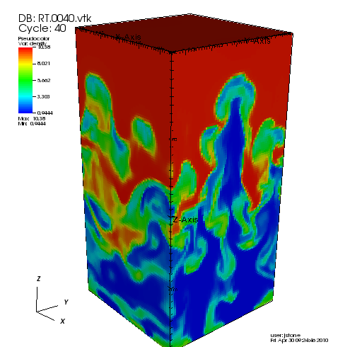
Only one history file will be created (in the id0 directory), and it will contain the data correctly integrated over the whole volume. To plot the vtk files, it may be necessary to join them together into one file at every time, there is a program /athena/vis/vtk/join_vtk.c that can do this. Below is an image of the density created by joining the vtk files and reading them with VisIt. Alternatively, VisIt is smart enough to join all the vtk files together automatically if each file from each directory is read individually.
Another good example to try running with MPI is the 3D linear wave convergence tests. Try configuring and compiling the code with MPI for this test, and then try running the code at different resolutions, and using different numbers of processors, to measure how the errors change with resolution.