Merging (and Unmerging) probability values

In quantum computing, it is common to end up with extremely large probability vectors, with relatively few states being interesting (having non-zero values). Dealing with the entire probability vector is thus not only memory-intensive, but also unhelpful in analysis/visualization (try plotting a 2^30 probability vector - not only will you run out of memory, you’ll see nothing in the resulting plot). The problem is compounded when these individually large probability vectors are combined (taking a Kronecker product of these vectors, for example, as is one in the cutqc2 codebase).

This notebook introduces the merge_prob_vector (and the corresponding unmerge_prob_vector) functions, the building blocks of classical postprocessing using cutqc2.

Merging

The merge_prob_vector function in cutqc2.utils takes in a probability vector and a qubit_spec - a string with characters that mean something specific:

• A - keep this qubit active, i.e. treat it as normal

• M - merge this qubit, i.e. sum the probability values for cases when this qubit is either 0 or 1. This effectively compresses multiple states into bins.

• 0 - only consider cases when this qubit is 0, otherwise, ignore them.

• 1 - only consider cases when this qubit is 1, otherwise, ignore them.

The merge operation thus returns a new probability vector (of length <= the original uncompressed vector), allowing us zoomed-in access to probability values.

Unmerging

The unmerge_prob_vector function does the opposite. It takes a compressed probability vector, the qubit_spec used to create it, and spreads the values across all possible states, distributing probability mass evenly when it needs to.

The unmerge operation thus returns a new probability vector (of length >= the compressed vector), allowing us zoomed-out access to probability values.

unmerge_prob_vector is obviously a lossy operation (since it assumes an even distribution between possible states), and cannot recover the original probability distribution.

The combined effect of merging/unmerging is that we get a blurred representation of the probability distribution.

Let’s see these in action.

import numpy as np
from matplotlib import pyplot as plt

from cutqc2.core.utils import merge_prob_vector, unmerge_prob_vector

(INFO) (base_tasks.py) (29-Sep-25 19:18:48) Pass: UnrollCustomDefinitions - 0.07272 (ms)
(INFO) (base_tasks.py) (29-Sep-25 19:18:48) Pass: BasisTranslator - 0.01788 (ms)

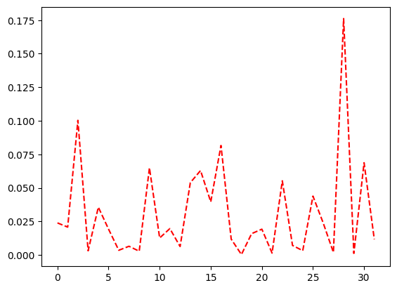
Create a length 32 (5 bit) probability vector using numpy, and plot it.

full_distribution = np.random.dirichlet(np.ones(32), size=1)[0]

plt.plot(range(len(full_distribution)), full_distribution, linestyle="--", color="r")

[<matplotlib.lines.Line2D at 0x7202eedb9b50>]

Let’s create a function that takes in the original distribution, a qubit_spec, and plots the distribution as well as the blurred representation of it (by merging and unmerging using the same qubit_spec).

def plot(dist, qubit_spec: str):
    # Plot original distribution
    plt.plot(range(len(dist)), dist, linestyle="--", color="r")

    # Plot coarse-grained distribution
    dist = unmerge_prob_vector(merge_prob_vector(dist, qubit_spec), qubit_spec)
    plt.bar(range(len(dist)), dist)
    plt.title(qubit_spec)
    plt.show()

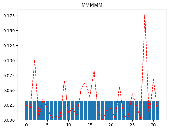
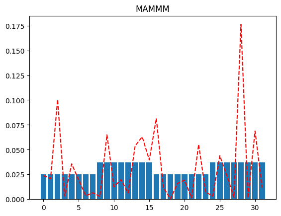
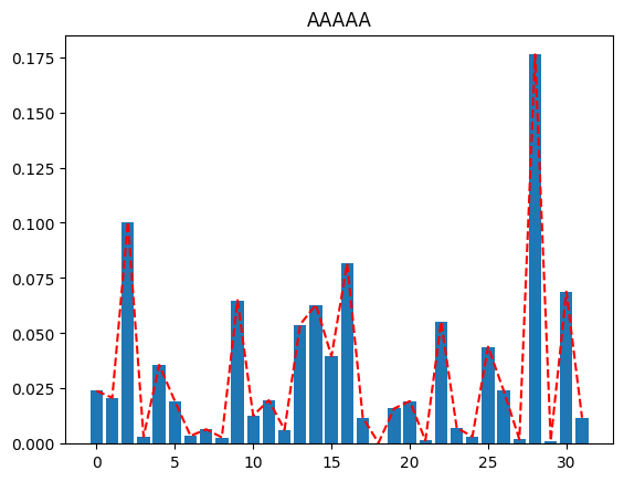
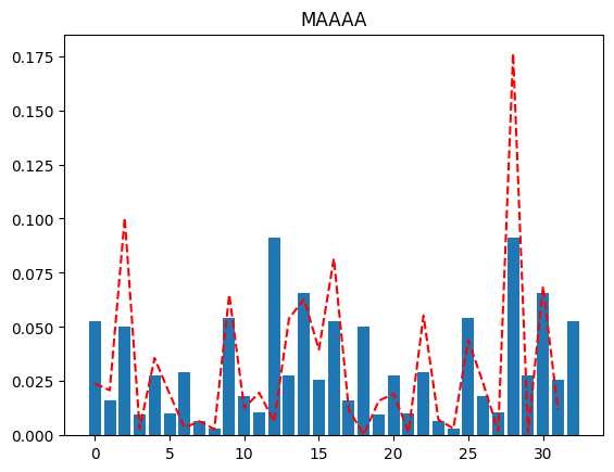
Look at the different plots we get for differing values of qubit_specs, going from all merged qubits (MMMMM) to all active (AAAAA). The more active qubits we have in our qubit_spec, the better the reconstructed distribution approximates the original distribution.

plot(full_distribution, "MMMMM")

plot(full_distribution, "MMMAM")
# note that the location of the active qubits matter.
# The following is not the same case as above.
plot(full_distribution, "MAMMM")

plot(full_distribution, "MAAAA")
plot(full_distribution, "AAAAA")

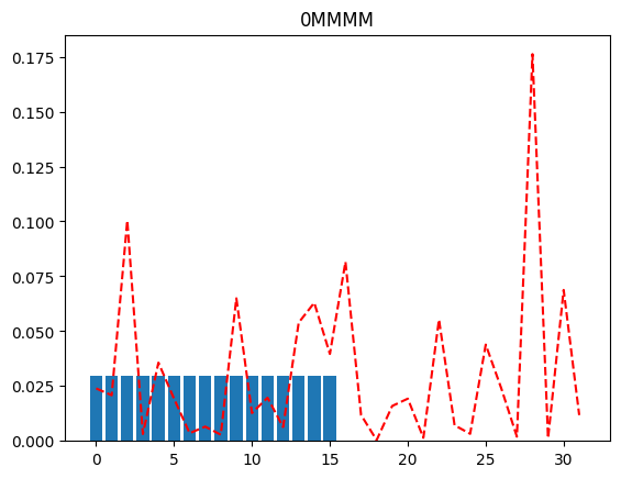
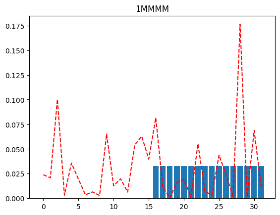
If we were peeking into the distribution using just a single qubit resolution, we might, as an example, try to plot the distribution when the MSB is 0 (and the rest of the qubits are merged), and again when the MSB is 1 (and the rest of the qubits are merged). This will tell us which half of the distribution has more probability mass (for further investigation).

plot(full_distribution, "0MMMM")
plot(full_distribution, "1MMMM")

Doesn’t unmerging undermine the whole point of doing all of this?

It is absolutely correct that unmerging like we’re naively doing here brings us back to the regime of 2^num_qubits address space. All the bar plots above have 32 bins after all. However, this is done here only for illustrative purposes. We will typically be using the unmerge_prob_vector function by passing in another argument, full_states, which is an ndarray of state values we’re interested in exploring.

Let us modify our plot function so it takes a full_states argument that we pass on to unmerge_prob_vector. We’ll call it selective_plot.

def selective_plot(dist, qubit_spec: str, full_states: np.ndarray):
    # Plot original distribution
    plt.plot(range(len(dist)), dist, linestyle="--", color="r")

    # Plot coarse-grained distribution
    dist = unmerge_prob_vector(
        merge_prob_vector(dist, qubit_spec), qubit_spec, full_states
    )
    plt.bar(range(len(dist)), dist)
    plt.title(qubit_spec)
    plt.show()

With this function, if we choose to work with 4 qubits (i.e. one merged and 4 active), we can choose to only expand the second half of the unmerged plot.

selective_plot(full_distribution, "MAAAA", np.arange(32, 65))

Conclusion

We’re now effectively able to approximate the original distribution of 5 qubits with a memory space of 4 qubits. The quality of the approximation may not be great (we’ll never know since we don’t have access to the original distribution - the dashed red lines in this toy example). That’s where the DynamicDefinition class comes in!