EXTENDER
The EXTENDER code (M. Drevlak, D. Monticello and A. Reiman. "PIES free boundary stellarator equilibria with improved initial conditions." Nuclear Fusion, 45 (2005)) uses a virtual casing principle (V.D. Shafranov and L.E. Zakharov. "Use of the virtual-casing principle in calculating the containing magnetic field in toroidal plasma systems." Nuclear Fusion 12 (1972)) to solve for the fields at a point in space due to a coil set and equilibrium (VMEC, PIES).
Theory
The EXTENDER code calculates the field of a given MHD equilibrium through a virtual casing principle. It can also be used to calculate a field due to a coils definition file. It is interfaced with the VMEC, PIES and HINT codes and can process their output files. Output from the code can either be the fields at a point in space (provided by the user) or on a set of grid planes in a style similar to the MAKEGRID code. This field can either be the total field, field due to coils or the plasma field alone.
The code utilizes a virtual casing principle when calculating the field due to a given plasma equilibrium. This is achieved through an invocation of Gauss's law, allowing the currents inside the equilibrium domain to be represented by a surface currents (and dipole moment densities) on the boundary of the equilibrium.
math \vec{K}=-\frac{1}{\mu_0}\hat{n}\times\vec{B} math math \rho_{dipole}=-\hat{n}\cdot\vec{B} math where the surface normal vector (n) is directed from the interior of the boundary toward the exterior and the magnetic field is taken to be that on the surface of the equilibrium. In order to find the field exterior to the equilibrium the surface current density (and dipole moment density) must be integrated over the entire surface. math \vec{B}_{ext}=\frac{\mu_0}{4\pi}\int\frac{\vec{K}'\times\left(\vec{x}-\vec{x}'\right)}{|\vec{x}-\vec{x}'|\^3}dA'+\frac{\mu_0}{4\pi}\int\frac{\rho_{dipole}'\left(\vec{x}-\vec{x}'\right)}{|\vec{x}-\vec{x}'|\^3}dA' math where the primes indicate quantities evaluated on the surface. For VMEC equilibria the normal field on the boundary is identically zero and the second term vanishes. Integration over the boundary is treated with a Newton-Cotes method allowing for treatment of points arbitrarily close to the surface. Calculation of the fields due to a set of field coils is conducted using a novel Biot-Savart's method.
Compilation
The EXTENDER code uses a make script to compile the code. The code requires NAG libraries, netCDF libraries, and MPI libraries. EXTENDER is written in C++ and has made extensive use of MPI and object oriented programming.
Input Data Format[[#Input]]
The EXTENDER code uses command line arguments to control input
EXTENDER -p <PIES FILE> -v <VMEC FILE> -vmec2000 <VMEC FILE> -vmec_netcdf <VMEC_FILE> -vmec_nyquist <VMEC FILE> -vmec93 <VMEC FILE>
-b <SURFACE FILE> -c <COILS FILE> -i <CONTROL FILE> -NU <POLOIDAL POINTS> -NV <TOROIDAL POINTS> -NI <NEWTON COTES INTERVALS> -NAIO <SOLVER>
-ps <PIES SURFACE> -s <SUFFIX> -rel <RELATIVE ERROR> -abs <ABSOLUTE ERROR> -points <POINTS FILE>
-plasmafield -full
|| Argument || Default || Description || || -p || || PIES netCDF file defining equilibrium || || -v || || VMEC wout file || || -vmec2000 || || VMEC2000 wout file || || -vmec_netcdf || || VMEC wout file (netCDF) || || -vmec_nyquist || || VMEC wout file (nyquist netCDF) || || -vmec93 || || VMEC93 wout file || || -b || Full Grid || Surface file containing the Fourier coefficients (mu+nv) defining the boundary. || || -c || NONE || Coils file - NOTE: The EXTENDER codes reads in the current for each filament from the 4th column of the Coils file. || || -i || || Control file defining number of radial and vertical points on grid, number of toroidal cut planes, maximum and minimum radial extend and maximum vertical extent || || -NU || 120 || Number of poloidal mesh points for surface integration || || -NV || 120 || Number of toroidal mesh points for surface integration (per half field period is stellarator symmetry can be assumed) || || -NI || 3 || Number of Newton-Cotes intervals to be replace by adaptive integration || || -NAIO || 4 || Order for adaptive integration || || -s || NONE || Suffix which is appended to output files || || -rel || 3E-7 || Relative error for adaptive integration || || -abs || 1E-10 || Absolute error for adaptive integration || || -points || NONE || File specifying a set of points in r, phi and z on which to calculate the field. || || -plasmafield || || Signals the code to calculate the field due to the plasma only. If a coils file is supplied the field inside the equilibrium is calculated by subtracting the vacuum field from the equilibrium solution. If no coils file is supplied, EXTENDER uses virtual casing to solve for the vacuum field inside the domain. The first method is considered more accurate. || || -full || || Computes the extended field on the whole domain (NOT recommended when computing the total field) || In it's simplest invocation the code requires an equilibrium output (PIES/VMEC/HINT) and will calculate the field on a grid.
The surface file (-b option) defines an outer boundary in terms of Fourier coefficients in NESCOIL format (mu+nv). If the extent of the grid is not specified in the control file (-i option) then this boundary file is used to determine the Rmin, Rmax, and Zmax values. Here is an example file which defines a circle of radius 0.5 centered at R=1.5:
# m   n           cr               cz
  0   0     1.5000000000e+00     0.0000000000e+00
  1   0     0.5000000000e+00     0.5000000000e+00
# Comments may be placed in any line
The control file specifies the grid parameters (number of radial points, number of vertical points, number of toroidal cut planes) it's format is as follows:
nr 130   # number of radial grid points
nz 120   # number of vertical grid points
nphi 110 # number of toroidal cut planes, never be fooled to believe you can save too much on nphi
rmin 4.0 # optional param., can be computed autom. from boundary
rmax 7.0 # optional parameter
zmax 1.3 # optional parameter
If the user wishes the field to be evaluated at a series of points in space then they simply must provide a pointsfile (-points option). The points are specified in x y and z:
# X     Y      Z
 1.5   0.0    0.0
 2.0   0.0    0.0
 2.5   2.5    0.0
Execution
The EXTENDER code is executed via the mpirun command and command line arguments are passed in order to determine the mode of execution. For example to run the code on 4 processors for a VMEC2000:
> mpirun -np 4 ./bin/EXTENDER -vmec2000 wout.test -i extender_in.test -c coils.test_machine -NU 360 -NV 72 -s test
Output Data Format
The extender code outputs two files by default called extended_mesh and extended_field. Passing the -s option will append a suffix to these files when output. The extended_mesh file contains information about the grid produced by EXTENDER. The extended_field file contains information about the fields on the grid. Both are text files.
The extended_mesh File
(taken from the ONSET User Guide) The mesh describes a domain of toroidal topology. Stellarator symmetry is assumed and hence only one half of one period is represented. The mesh consists of cells, retangular in (r,phi,z), delimited by points. Points and cells are located equidistantly in (r,phi,z). The mesh assumes points located in the range math \left(\left[r_{min},r_{max}\right],\left[0,\pi/N_{per}\right],\left[-z_{max},z_{max}\right]\right) math Of these points, a continuous subset is used for representing fields. Hence, fields can be made to fit into distorted 3d domains, like the interior of a coil set. Therefore, meshes are generated using a toroidal surface selecting the region from which points arre to be used. A point/cell belonging to the continuous subset is called active, outside points/cells, are inactive. The mesh file contains the data marking points/cells as active or inactive and provides the auxiliary data for addressing the active points/cells in a continuous memory space. The surface selecting the active region will, in general, cut through cells located at the edge of the domain. In order to complete these cells, points just outside the selecting surface will be added to the domain and marked as active. These points will be called boundary points. Points inside the domain are inner points. Points are assigned indicies in their corrdinates, i, j,k, relating to their position as math r=r_{min}+\Delta r \frac{i}{\left(N_r-1\right)},i=0...N_r-1 math math \phi=\frac{\pi}{N_{per}}\frac{j}{\left(N_\phi-1\right)},j=0...N_\phi-1 math math z=-z_{max}+\Delta z \frac{k}{\left(N_z-1\right)},k=0...N_z-1 math The coordinate indicies for cells, in contrast to those of points, range between [0...Nr-2], [0...Nphi-2], and [0...N_z-2]. In order to map the entire set of points, active and inactive, onto a linear indexing space, they are assigned the total indicies math i_P=i+jN_r+kN_rN_\phi math Likewise, cells are indexed as math i_C=i+j\left(N_r-1\right)+k\left(N_r-1\right)\left(N_\phi-1\right) math A mesh file typically looks like this
ConstrainedGeometry
1568000 1526359
1.92547 1.5708 2.30319
0.904265 2.82973 1.15159
2
140 80 140
531728 561157
45297 515860
0 -1
0 -1
0 -1
0 -1
.
.
.
591883
591884
591885
591886
591887
591888
591889
591890
591891
591892
591893
.
.
.
The data printed are:
- An identifier of the file contents, ConstrainedGeometry
- Number of points Np, number of cells Nc, both active and inactive
- Rmax-Rmin, pi/Nper, 2*Zmax
- Rmin,Rmax,Zmax
- Nper
- Number of steps of the mesh Nr, Nphi, Nz
- Number of active points Npa, number of active cells Nca
- Number of boundary points Nb, number of interior points Ni
- Np lines, containing > (a) integer flag marking activity of each points > (b) address of point in linear address space, -1 if inactive
- Nc lines, containing > (a) integer flag marking activity of each cell > (b) address of cell in linear address space, -1 if inactive
- Npa lines, indicies of active points
- Nca lines, indicies of active cells
The extended _field File
The field file holds the cylindrical components of a vector field at the points marked active by the mesh. A field file typically looks like this:
ConstrainedVField
561157
2
140
80
140
0.904265
2.82973
1.15159
0.056905
0.0563255
0.0557642
0.0552217
0.0546985
0.0541949
0.0537116
0.0532488
.
.
.
The data printed are:
- An identifier of the file contents, ConstrainedVField
- Number of active points Npa
- Number of periods Nper
- Number of radial points Nr
- Number of poloidal points Nphi
- Number of axial points Nz
- Minimum radius rmin
- Maximum radius rmax
- Maximum elevation zmax
- Npa lines, radial components of field at active points (Hr)
- Npa lines, poloidal components of field at active points (Hphi)
- Npa lines, axial components of field at active points (Hz)
The points File
If the user requested the field be evaluated at a set of points (-points option) then an output will be generated with the same name as the points file with 'out' as a suffix (eg. -p b_test, b_test.out). This is a text file with the following format:
#  i      r               phi             z               H_r             H_phi           H_z             |H|            inside
       0  4.80242700e+00  6.14355900e+00  4.30900000e-01 -7.86465604e+03 -1.00325890e+03  1.22797224e+04  1.46168028e+04 0
       1  4.63074100e+00  6.10865200e+00  5.10120000e-01 -1.69277773e+04 -3.76178271e+03  1.23201685e+04  2.12717466e+04 0
       2  4.22074400e+00  6.03883900e+00  6.15140000e-01 -3.50921255e+04 -2.06069275e+03 -1.56921383e+04  3.84960639e+04 0
Here the output values are in terms of magnetic induction and must be multiplied by mu0.
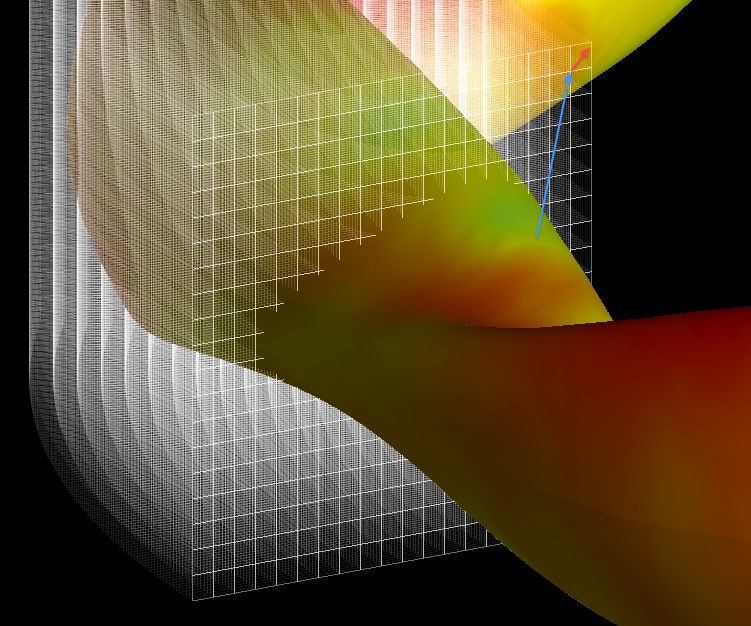
Visualization
Visualization of the extender output can be preformed similar to that of a MAKEGRID file. A visualization package exists in MATLAB to facilitate plotting of the fields (matlabEXTENDER, http://www.mathworks.com/matlabcentral/fileexchange/31470).