FIELDLINES
Table of Contents
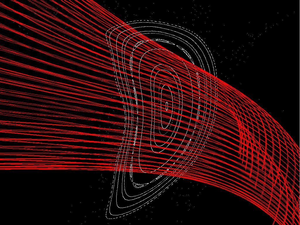
The FIELDLINES code follows field lines in a toroidal domain given a vacuum, VMEC, PIES, or SPEC equilibria, and is parallelized over the field line trajectories.
Theory
The FIELDLINES code follows fieldlines in a toroidal domain. This is achieved by placing the magnetic field on an R-phi-Z mesh and constructing splines over that mesh. An ODE for following field lines as a function of the toroidal angle can be constructed by relating the motions in R and Z as a function of phi through
\(\frac{\partial R}{\partial \phi} = R\frac{B_R}{B_\phi}\) and \(\frac{\partial Z}{\partial \phi} = R\frac{B_Z}{B_\phi}\)
In this representation the trajectory of the fieldline can be
parameterized by toroidal angle. The resulting ODE is solved with a user
determined step-size and accuracy. The available ODE packages are:
LSODE,
NAG D02CJF(requires
license), and a Runge-Kutta-Hutta 6-th order 8 step method
(D. Sarafyan, J. Math. Anal. Appl. 40, 436-455 (1972))
. The calculation of field line trajectories is parallelized over each
field line. Thus each processor can follow each field line independently
to speed computation. It should be noted that PHI_END and PHI_START
define the direction of integration. The -reverse flag is present to
aide in switching the sign of PHI_END automatically.
The code assembles fields from various sources. The vacuum component of the field can be calculated directly from a coils file or an mgrid file. In the later case the FIELDLINES grid must match the mgrid file. The plasma field inside the equilibria domain is placed directly on the background grid. The plasma response external to the equilibria is calculated using a virtual casing principle. In order to maintain accuracy near the surface of the plasma, the virtual casing principle employs an adaptive integration scheme over the surface current. This scheme is either handled by NAG D01EAF (if available), or the DCUHRE algorithm (J. Berntsen, T. O. Espelid and A. Genz, Trans. Math. Softw. 17 (1991), pp. 437-451., J. Berntsen, T. O. Espelid and A. Genz, Trans. Math. Softw. 17 (1991), pp. 452-456.) . This part of the code is parallelized over the vertical dimension (Z). Thus the z-axis is domain decomposed.
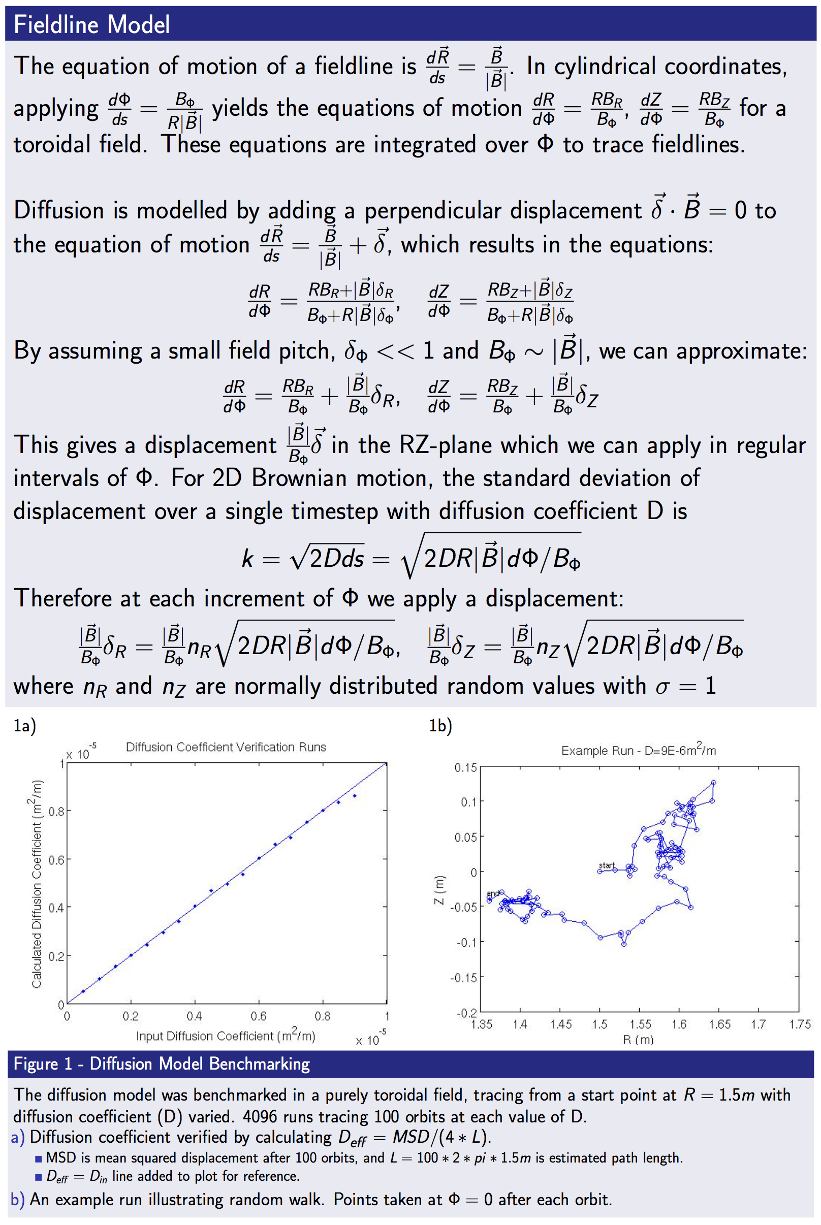
The code can also be given a limiting surface (vessel, first wall, divertor). Field lines which pass through this surface are not followed beyond that point. An artificial diffusion can also be applied to aid in modeling divertor strike points.
If the user wishes, the code can automatically locate the magnetic axis, find the 'edge' of the flux surfaces, and output the periodic orbit of the edge with the -full option. Here the code begins by first following fieldlines from the minimum and maximum values in R_START and Z_START. A magnetic axis is identified using a periodic orbit search. The edge is then refined once so any edge stochastic region may be resolved. The code then follows fieldlines in this domain from the axis to the 'edge.' If the user supplies an R,PHI,Z guess for the edge periodic orbit the code will find it and the associated separatrix.
Compilation
FIELDLINES is a component of the STELLOPT suite of codes.
Input Data Format
The FIELDLINES code is controled through command line inputs and an input namelist which should be placed in the input.ext file. While the entire VMEC input name is not required the EXTCUR array is required. The name lists should look like:
#!fortran
&INDATA
 ! VMEC input namelist (only need coil currents for usual runs)
 EXTCUR(1) = 10000.00
 EXTCUR(2) = 10000.00
 EXTCUR(3) = 12000.00
 EXTCUR(4) = 12000.00
 EXTCUR(5) = 6000.00
 ! VMEC Axis info (for putting a current on axis -axis option)
 !     This information is utilized if you want to place the net toroidal current
 !     on a magnetic axis.  Useful for doing vacuum tokamak equilibria
 CURTOR = 5000.0
 NFP = 5
 NTOR = 6
 RAXIS = 3.6  0.1 0.001
 ZAXIS = 0.0  0.1 0.001
/
&FIELDLINES_INPUT
!---------- Background Grid Parameters ------------
 NR = 251                          ! Number of radial gridpoints
 NPHI = 36                         ! Number of toroidal gridpoints
 NZ = 301                          ! Number of vertical gridpoints
 RMIN = 2.5                        ! Minimum extent of radial grid
 RMAX = 5.0                        ! Maximum extent of radial grid
 ZMIN = -1.5                       ! Minimum extent of vertical grid
 ZMAX = 1.5                        ! Maximum extent of vertical grid
 PHIMIN = 0.0                      ! Minimum extent of toroidal grid, overridden by mgrid or coils file
 PHIMAX = 0.628                    ! Maximum extent of toroidal grid, overridden by mgrid or coils file
 VC_ADAPT_TOL = 1.0E-7             ! Virtual casing tolerance (if using plasma field from equilibria)
!---------- Magnetic Material Parameters ----------
 MUMATERIAL_NITER = 1000           ! Maximum number of iterations in magnetization solve
 MUMATERIAL_TOL   = 1.0E-5         ! Error Threshold
 MUMATERIAL_LAMTHRESH = 10         !
 MUMATERIAL_LAMBDA    = 0.7        ! Damping Factor for Picard Iteration
 MUMATERIAL_LAMFACTOR = 0.75       !
 MUMATERIAL_PADFACTOR = 0.3        ! Factor of NN in terms of total domain
 MUMATERIAL_CONVCHECK = 99.0       ! Convergence Check in %
!---------- Marker Tracking Parameters ------------
 INT_TYPE = 'LSODE'                ! Fieldline integration method (NAG, RKH68, LSODE)
 FOLLOW_TOL = 1.0E-12              ! Fieldline ODE solver tollerance
 NPOINC = 72                       ! Number of toroidal points per-period to output the field line trajectory
 MU = 0.0                          ! Fieldline diffusion (mu=D/v) [m^2/m]
 R_START =  3.6  3.7  3.8          ! Radial starting locations of fieldlines
 Z_START =  0.0  0.0  0.0          ! Vertical starting locations of fieldlines
 PHI_START =  0.0  0.0  0.0        ! Toroidal starting locations of fieldlines (radians)
 PHI_END =  629.0  629.0  629.0    ! Maximum distance in toroidal direction to follow fieldlines
!---------- Periodic Orbits (-full) ------------
 NUM_HCP = 512                     ! Number of points for separatrix plot (-full)
 DELTA_HC = 1.0E-4                 ! Initial length of separatrix line (-full)
 R_HC = 3.5                        ! R Location of periodic orbit (-full)
 Z_HC = 0.5                        ! Z Location guess for periodic orbit (-full)
 PHI_HC = 0.0                      ! PHI Location for periodic orbit(-full)
!---------- Error Fields ------------
 ERRORFIELD_AMP =   1.0E-4 0.0 0.0 ! Amplitude of analytic error field
 ERRORFIELD_PHASE = 1      2   3   ! Toroidal phase (n) of error field
/
&END
The toroidal background grid repeats the endpoint so that grid points
1 and NPHI are the same. To enforce the half field period point,
one should choose an odd number for number of gridpoints. The
following table outlines some common choices for 1 degree separation
| NPF | NPHI |
|---|---|
| 1 | 361 |
| 2 | 181 |
| 3 | 121 |
| 4 | 91 |
| 5 | 73 |
| 10 | 19 |
When modeling an NFP=1 system it is best to comment out PHIMAX as
this sets it to 2*pi at machine precision. It is important to remember
that if you system has an underlying stellarator symmetry you need to
carefully choose the number of grid points. The general rule is if you
want NPHI0 unique gridpoints per field period, then you need to set
NPHI = NPHI0*NFP+1. The following table should help
| NPF | 1 deg | Half res |
|---|---|---|
| 1 | 361 | 181 |
| 2 | 361 | 181 |
| 3 | 361 | 181 |
| 4 | 361 | 177 |
| 5 | 361 | 181 |
| 10 | 361 | 181 |
The MU diffusion coefficient has units of [m^2/m]. To convert the traditional diffusion coefficient D [m^2/s] to MU you simply divide D by the typical velocity (usually the sound speed) of your particle.
Execution
The FIELDLINES code is controlled through a combination of command-line inputs and an input namelist. The input namelist must be in the equilibrium input file. That file must also contain the VMEC INDATA namelist (although only the EXTCUR array will be used). The FIELDLINES code is run from the command line taking an equilibrium input file as a necessary argument. This input file must have the INDATA (for EXTCUR) and FIELDLINES_IN namelists in it.
XFIELDLINES -vmec <VMEC ID> -pies <PIES_FILE> -spec <SPEC FILE> -coil <COIL FILE> -mgrid <MGRID FILE> -vessel <VESSEL FILE> -vac -full -noverb -help
| Argument | Default | Description |
|---|---|---|
| -vmec | NONE | VMEC input extension |
| -hint | NONE | HINT input/magslice extension |
| -eqdsk | NONE | FIELDLINES input extension and gfile |
| -coil | NONE | Coils File |
| -mgrid | NONE | Makegrid style vacuum grid file |
| -nescoil | NONE | NESCOIL file (for vacuum) |
| -vessel | NONE | First wall file |
| -screen | NONE | Poincaré Screen file |
| -mumat | NONE | Magnetic materials mesh file |
| -mumat_magfile | NONE | Magnetic materials magnetization file |
| -mumat_skipiter | NONE | Skip iterations |
| -mumat_writemagfile | NONE | Write out magnetization file |
| -vac | NONE | Only compute the vacuum field |
| -raw | NONE | Treat vacuum field current in RAW format (EXTCUR as scaling factor) |
| -plasma | NONE | Plasma field only |
| -field | NONE | Outputs the B-Field on the cylindrical grid only. |
| -vecpot | NONE | Outputs the vector potential on the cylindrical grid only. |
| -emc3 | NONE | Output EMC3 Grid (very experimental) |
| -gridgen | NONE | Create a fieldline grid for BEAMS3D. |
| -modb | NONE | Save mod(B) along fieldline. |
| -field_start | NONE | Extension and fieldline number to use for initializing run. |
| -auto | NONE | Starting points set equal to radial grid and run from the min to max values of R_START and Z_START |
| -full | NONE | Auto calculate axis and edge maximum resolution |
| -hitonly | NONE | Only save strikepoint locations (used in conjunction with -vessel) |
| -reverse | NONE | Follow particles in oposite direction. |
| -edge | NONE | Place all starting points at VMEC boundary. |
| -noverb | NONE | Suppresses screen output |
| -help | NONE | Print help message |
In it's simplest invokation the code requires a VMEC input file and some source of vacuum field. Please note that FIELDLINES takes advantage of shared memory MPI so the user must request full nodes
>mpirun -N 6 ~/bin_847/xfieldlines -vmec ncsx_c09r00_free -mgrid mgrid_c09r00.nc -vac
FIELDLINES Version 0.50
----- Input Parameters -----
   FILE: input.ncsx_c09r00_free
   R   = [ 0.43600, 2.43600];  NR:    201
   PHI = [ 0.00000, 2.09440];  NPHI:   36
   Z   = [-1.00000, 1.00000];  NR:    201
   # of Fieldlines:   40
   VACUUM FIELDS ONLY!
----- MGRID Information -----
   FILE:mgrid_c09r00.nc
   R   = [ 0.43600, 2.43600];  NR   =  201
   PHI = [ 0.00000, 2.09440];  NPHI =   37
   Z   = [-1.00000, 1.00000];  NZ   =  201
----- FOLLOWING FIELD LINES -----
      Method: NAG
       Lines:   40
         Tol: 0.1000E-08  Type: M
   Delta-phi: 0.1745E-01
       Lines:  359989
----- WRITING DATA TO FILE -----
   FILE: fieldlines_ncsx_c09r00_free.h5
----- FIELDLINES DONE -----
Output Data Format
The FIELDLINES code outputs data in the HDF5 data format. The trajectory of each field line and relevant quantities for each run are stored in a fieldline_ext.h5 file. A MATLAB routine for reading the HDF5 file is available (MATLAB File Exchange: read_fieldlines.m). A sample of the HDF5 data structure looks like:
HDF5 "fieldlines_ncsx_c09r00_free.h5" {
GROUP "/" {
   DATASET "B_R" {
      DATATYPE  H5T_IEEE_F64LE
      DATASPACE  SIMPLE { ( 201, 36, 201 ) / ( 201, 36, 201 ) }
   }
   DATASET "B_Z" {
      DATATYPE  H5T_IEEE_F64LE
      DATASPACE  SIMPLE { ( 201, 36, 201 ) / ( 201, 36, 201 ) }
   }
   DATASET "PHI_lines" {
      DATATYPE  H5T_IEEE_F64LE
      DATASPACE  SIMPLE { ( 359990, 40 ) / ( 359990, 40 ) }
   }
   DATASET "R_lines" {
      DATATYPE  H5T_IEEE_F64LE
      DATASPACE  SIMPLE { ( 359990, 40 ) / ( 359990, 40 ) }
   }
   DATASET "Z_lines" {
      DATATYPE  H5T_IEEE_F64LE
      DATASPACE  SIMPLE { ( 359990, 40 ) / ( 359990, 40 ) }
   }
   DATASET "lcoil" {
      DATATYPE  H5T_STD_I32LE
      DATASPACE  SIMPLE { ( 1 ) / ( 1 ) }
   }
   DATASET "lmgrid" {
      DATATYPE  H5T_STD_I32LE
      DATASPACE  SIMPLE { ( 1 ) / ( 1 ) }
   }
   DATASET "lmu" {
      DATATYPE  H5T_STD_I32LE
      DATASPACE  SIMPLE { ( 1 ) / ( 1 ) }
   }
   DATASET "lpies" {
      DATATYPE  H5T_STD_I32LE
      DATASPACE  SIMPLE { ( 1 ) / ( 1 ) }
   }
   DATASET "lspec" {
      DATATYPE  H5T_STD_I32LE
      DATASPACE  SIMPLE { ( 1 ) / ( 1 ) }
   }
   DATASET "lvac" {
      DATATYPE  H5T_STD_I32LE
      DATASPACE  SIMPLE { ( 1 ) / ( 1 ) }
   }
   DATASET "lvessel" {
      DATATYPE  H5T_STD_I32LE
      DATASPACE  SIMPLE { ( 1 ) / ( 1 ) }
   }
   DATASET "lvmec" {
      DATATYPE  H5T_STD_I32LE
      DATASPACE  SIMPLE { ( 1 ) / ( 1 ) }
   }
   DATASET "nlines" {
      DATATYPE  H5T_STD_I32LE
      DATASPACE  SIMPLE { ( 1 ) / ( 1 ) }
   }
   DATASET "nphi" {
      DATATYPE  H5T_STD_I32LE
      DATASPACE  SIMPLE { ( 1 ) / ( 1 ) }
   }
   DATASET "npoinc" {
      DATATYPE  H5T_STD_I32LE
      DATASPACE  SIMPLE { ( 1 ) / ( 1 ) }
   }
   DATASET "nr" {
      DATATYPE  H5T_STD_I32LE
      DATASPACE  SIMPLE { ( 1 ) / ( 1 ) }
   }
   DATASET "nsteps" {
      DATATYPE  H5T_STD_I32LE
      DATASPACE  SIMPLE { ( 1 ) / ( 1 ) }
   }
   DATASET "nz" {
      DATATYPE  H5T_STD_I32LE
      DATASPACE  SIMPLE { ( 1 ) / ( 1 ) }
   }
   DATASET "phiaxis" {
      DATATYPE  H5T_IEEE_F64LE
      DATASPACE  SIMPLE { ( 36 ) / ( 36 ) }
   }
   DATASET "raxis" {
      DATATYPE  H5T_IEEE_F64LE
      DATASPACE  SIMPLE { ( 201 ) / ( 201 ) }
   }
   DATASET "zaxis" {
      DATATYPE  H5T_IEEE_F64LE
      DATASPACE  SIMPLE { ( 201 ) / ( 201 ) }
   }
}
}
Visualization
A command line tool for visualizing FIELDLINES data is provided called
fieldlines_util.py. It is installed when you install the pySTEL
library included with STELLOPT.
Tutorials
FIELDLINES Vacuum NCSX Tutorial
References
- Lazerson, S.A. et al. "First measurements of error fields on W7-X using flux surface mapping" Nuclear Fusion 56, 106005 (2016)
- Lazerson, S.A. et al. "Error field measurement, correction and heat flux balancing on Wendelstein 7-X" Nuclear Fusion 56, 046026 (2017)
- Lazerson, S.A. et al. "Error fields in the Wendelstein 7-X stellarator" Plasma Phys. Control. Fusion 60, 124002 (2018)
- Lazerson, S.A. et al. "Tuning of the rotational transform in Wendelstein 7-X" Nuclear Fusion 59, 126004 (2019)
- Engels, D. et al. "Investigating the n=1 and n=2 error fields in W7-X using the newly accelerated FIELDLINES code" Plasma Phys. Control. Fusion (accepted) (2022)