Synthetic HI 21cm lines#
import matplotlib.pyplot as plt
import numpy as np
# add path to astro_tigress module
# this can also be done using PYTHONPATH environment variable
import sys
sys.path.insert(0,'../')

import astro_tigress
# Need to set the master directory where the data is stored
dir_master = "../data/"
# name of the simulation model
model_id = "R8_4pc"
model = astro_tigress.Model(model_id,dir_master) #reading the model information
Download the data if you haven’t done it yet
You can navigate the folder and only download selected snapshots.
You will always need
histroyandinputfiles. You can run the following.
    model.download(dataset=["history","input"])
    model = astro_tigress.Model(model_id,dir_master) # need to reload the class
#load the MHD data set for the snapshot ivtk=300
model.load(300, dataset="MHD")
Because we use the python package YT to read the outputs from the MHD simulation, the data stored in the YT format. This means that all fields (such as density, velocity, H2 and CO abundances) in the data has units atached.
Let’s convert the YT covering grid into numpy arrray with appropriate units. Also, I take transpose so that the array is in the original C-like ordering (z,y,x)
Temp = model.MHD.grid[('gas','temperature')].in_units("K").value.T
nH = model.MHD.grid[('gas','nH')].in_units("cm**-3").value.T
vx = model.MHD.grid[('gas','velocity_x')].in_units("km/s").value.T
vy = model.MHD.grid[('gas','velocity_y')].in_units("km/s").value.T
vz = model.MHD.grid[('gas','velocity_z')].in_units("km/s").value.T
Retrieve cell-centered coordinates for later uses.
xcc = model.MHD.grid[("gas","x")][:,0,0].to('pc').value
ycc = model.MHD.grid[("gas","y")][0,:,0].to('pc').value
zcc = model.MHD.grid[("gas","z")][0,0,:].to('pc').value
Get cell size in pc and cm for convenience (note that the cell is cubic)
dx_pc = model.MHD.grid[("gas","dx")][0,0,0].to('pc').value
dx_cm = model.MHD.grid[("gas","dx")][0,0,0].to('cm').value
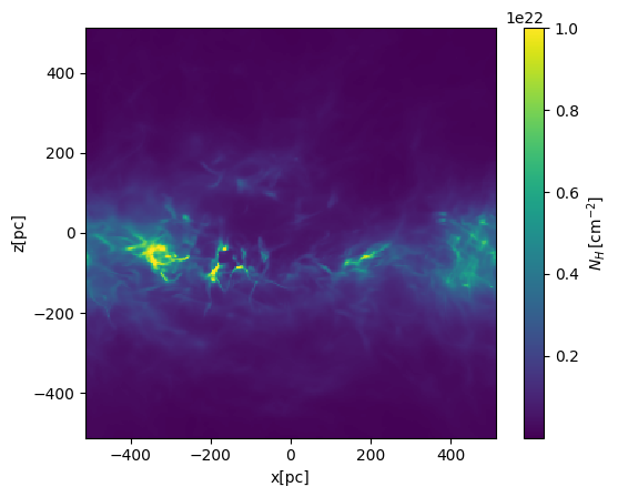
Column density projection (along the y-direction)#
# integration along the y-axis (edge on view)
NH = nH.sum(axis=1)*dx_cm
plt.pcolormesh(xcc,zcc,NH,vmax=1.e22,shading='nearest')
plt.gca().set_aspect('equal')
plt.xlabel('x[pc]')
plt.ylabel('z[pc]')
cbar = plt.colorbar(label=r'$N_H\,[{\rm cm^{-2}}]$')
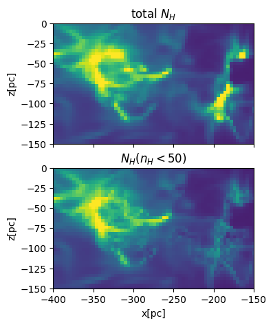
Maybe some dense gas is molecular (n>50pcc)#
# set threshold density to exclude (assuming that they are molecular)
nth_mol = 50

# integration along the y-axis (edge on view)
NH = nH.sum(axis=1)*dx_cm

# integration along the y-axis excluding molecular gas
nH_masked=nH*(nH<nth_mol) # np.ma.masked_array(nH,mask=nH>nth_mol)
NHI = nH_masked.sum(axis=1)*dx_cm

fig,axes = plt.subplots(2,1,figsize=(5,5),sharex=True,sharey=True)
plt.sca(axes[0])
plt.pcolormesh(xcc,zcc,NH,vmax=1.e22,shading='nearest')
plt.gca().set_aspect('equal')
plt.title('total $N_H$')
# plt.xlabel('x[pc]')
plt.ylabel('z[pc]')
plt.sca(axes[1])
plt.title('$N_H(n_H<50)$')
plt.pcolormesh(xcc,zcc,NHI,vmax=1.e22,shading='nearest')

plt.gca().set_aspect('equal')
plt.xlabel('x[pc]')
plt.ylabel('z[pc]')
plt.xlim(-400,-150)
plt.ylim(-150,0)
(-150.0, 0.0)
Synthetic HI#
Following the method presented in https://ui.adsabs.harvard.edu/abs/2014ApJ…786…64K/abstract
Assuming that the WF effect is efficient enough to make T_spin = T_k based on Ly alpha radiation transfer study https://ui.adsabs.harvard.edu/abs/2020ApJS..250….9S/abstract
- \[N_H = 1.813\times10^{18}{\rm cm^{-2}}\int T_B \frac{\tau}{1-e^{-\tau}} d(v/(km/s))\]
from astro_tigress.synthetic_HI import los_to_HI_axis_proj
help(los_to_HI_axis_proj)
Help on function los_to_HI_axis_proj in module astro_tigress.synthetic_HI:

los_to_HI_axis_proj(dens, temp, vel, vchannel, deltas=1.0, los_axis=1)
    inputs:
        dens: number density of hydrogen in units of 1/cm^3
        temp: temperature in units of K
        vel: line-of-sight velocity in units of km/s
        vchannel: velocity channel in km/s
    parameters:
        deltas: length of line segments in units of pc
        memlim: memory limit in GB
        los_axis: 0 -- z, 1 -- y, 2 -- x
    outputs: a dictionary
        TB: the brightness temperature
        tau: optical depth
# this will take some time

vmin,vmax,dv=-50,50,0.5
vch = np.arange(vmin,vmax+0.5*dv,dv) # velocity resolution of 0.5 km/s
nth_mol = 50 # threshold density above which gas is considered as H2
Tth = 1.5e4 # threshold temperature above which gas is considered as HII
nH_masked=nH*((nH<nth_mol) & (Temp<Tth))
TB,tau = los_to_HI_axis_proj(nH_masked,Temp,vy,
                             vch,deltas=dx_pc,
                             los_axis=1, # axis along which the integration is performed (0='z', 1='y', 2='x')
                            )
100%|██████████| 201/201 [03:01<00:00, 1.11it/s]
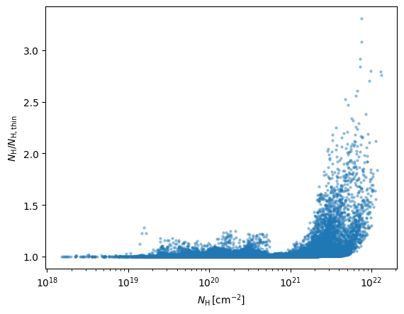
NHI = nH_masked.sum(axis=1)*dx_cm
NHthin = 1.813e18*TB.sum(axis=0)*dv
plt.plot(NHI.flatten(),NHI.flatten()/NHthin.flatten(),'.',alpha=0.5,mew=0)
plt.xscale('log')
plt.xlabel(r'$N_{\rm H}\,[{\rm cm^{-2}}]$')
plt.ylabel(r'$N_{\rm H}/N_{\rm H, thin}$')
Text(0, 0.5, '$N_{\\rm H}/N_{\\rm H, thin}$')
from astro_tigress.synthetic_HI import save_to_fits
help(save_to_fits)
Help on function save_to_fits in module astro_tigress.synthetic_HI:

save_to_fits(ytds, vchannel, TB, tau, axis='xyv', fitsname=None)
    Function warpper for fits writing

    Parameters
    ----------
    ytds: yt.Dataset
        yt Dataset
    vchannel: array
        velocity channel array
    TB: array
        PPV data cube for brightness temperature
    tau: array
        PPV data cube for optical depth
    axis: str
        str for the PPV coordniate names
    fitsname: str
        if not None, fits file is created
hdul=save_to_fits(model.MHD.ytds, vch, TB, tau, axis='xzv', fitsname='test.fits')
FITS file named test.fits is created
hdul[0].header
SIMPLE  =                    T / conforms to FITS standard
BITPIX  =                    8 / array data type
NAXIS   =                    0 / number of array dimensions
EXTEND  =                    T
TIME    =     293.337862012388
XMIN    =               -512.0 / pc
XMAX    =                512.0 / pc
YMIN    =               -512.0 / pc
YMAX    =                512.0 / pc
ZMIN    =               -512.0 / pc
ZMAX    =                512.0 / pc
DX      =                  4.0 / pc
DY      =                  4.0 / pc
DZ      =                  4.0 / pc
VMIN    =                -50.0 / km/s
VMAX    =                 50.0 / km/s
DV      =                  0.5 / km/s
CDELT1  =                  4.0
CTYPE1  = 'x       '
CUNIT1  = 'pc      '
CRVAL1  =               -512.0
CRPIX1  =                  0.0
CDELT2  =                  4.0
CTYPE2  = 'z       '
CUNIT2  = 'pc      '
CRVAL2  =               -512.0
CRPIX2  =                  0.0
CDELT3  =                  0.5
CTYPE3  = 'v       '
CUNIT3  = 'km/s    '
CRVAL3  =                -50.0
CRPIX3  =                  0.0
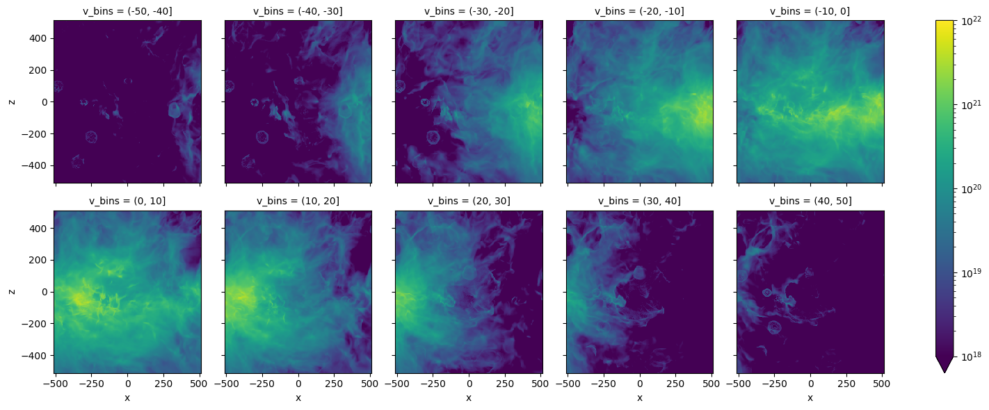
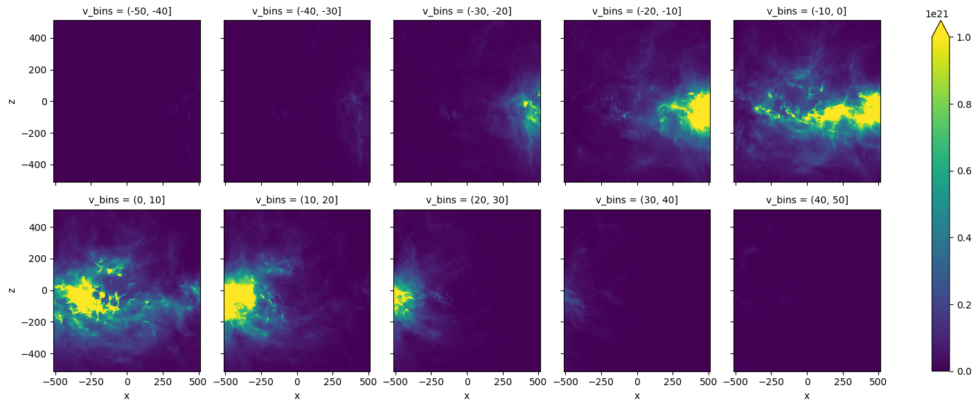
import xarray as xr
TB_da = xr.DataArray(TB,coords=[vch,zcc,xcc],dims=['v','z','x'])
NHthin=1.813e18*dv*TB_da.groupby_bins('v',np.arange(-50,51,10)).sum()
NHthin.plot(col='v_bins',col_wrap=5,vmax=1.e21)
<xarray.plot.facetgrid.FacetGrid at 0x13e326b50>
from matplotlib.colors import LogNorm
NHthin.plot(col='v_bins',col_wrap=5, vmin=1.e18, vmax=1.e22, norm=LogNorm())
<xarray.plot.facetgrid.FacetGrid at 0x1407ebbd0>