from scipy.interpolate import interp1d
import matplotlib.pyplot as plt
import numpy as np
import yt  # https://yt-project.org/
import sys

# add path to astro_tigress module
# this can also be done using PYTHONPATH environment variable
sys.path.insert(0, "../")

import astro_tigress  # noqa
Show code cell content
%load_ext autoreload
%autoreload 2
MHD datasets#
This script focus on reading and analysing the original MHD dataset from the original TIGRESS simulation run by the Athena4.2 code (Kim & Ostriker (2017)). The vertical dimension is trucated at \(z=\pm512{\rm pc}\)
Examining the simulation model information#
# Need to set the master directory where the data is stored
dir_master = "../data/"
# name of the simulation model
model_id = "R8_4pc"
First, we can look into what snapshots are available, and what types of datasets they contain.
Each snapshot has an “ivtk” number. This is the Athena4.2 VTK output id.
The time for each snapshot is ivtk*dt_Myr, where dt_Myr is the output interval per vtk number in Myr.
For the “R8_2pc” simulation, we release the data in the time frame when the simulation has already reached a steady state. The data release time interval is about 10 Myr.
# one can download a data snapshot using `download` method
# dataset can be one of ["MHD", "chem", "CO_lines", "history", "input", "all"]
model = astro_tigress.Model(model_id, dir_master)  # reading the model information
Download the data if you haven’t done it yet
You can navigate the folder and only download selected snapshots.
You will always need
histroyandinputfiles. You can run the following.
    model.download(dataset=["history","input"])
    model = astro_tigress.Model(model_id,dir_master) # need to reload the class
print("Snapshots and contained data sets:")
for ivtk in model.ivtks:
    print(
        "ivtk={:d}, t={:.1f} Myr, datasets={}".format(
            ivtk, ivtk * model.dt_Myr, model.data_sets[ivtk]
        )
    )
Snapshots and contained data sets:
ivtk=300, t=293.3 Myr, datasets=['Bfield', 'MHD', 'MHD_PI', 'RAD']
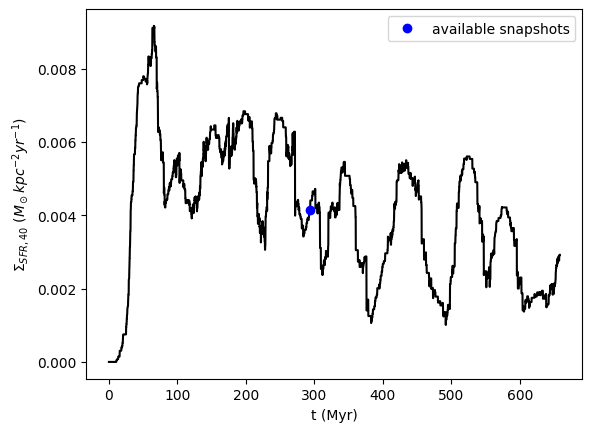
We can also look at the history output, which contains the overall information (such as the star formation rate) of the simulation as a function of time.
fig = plt.figure()
ax = fig.add_subplot(111)
# star formation rate (averaged over 40 Myr)
ax.plot(model.hst["time"] * model.tunit_Myr, model.hst["sfr40"], "k-")
# snapshots
f = interp1d(model.hst["time"] * model.tunit_Myr, model.hst["sfr40"])
ax.plot(model.t_Myr, f(model.t_Myr), "bo", label="available snapshots")
ax.legend()
ax.set_ylabel("$\Sigma_{SFR,40}\ (M_\odot kpc^{-2} yr^{-1})$")
ax.set_xlabel("t (Myr)")
Read and analyze the 3D MHD simulation output#
Now, we want to look into the detailed 3D simulation data of the simulations. First, we select a snapshot (identified by its ivtk number) and the type of dataset we want to look into (“MHD” in this case). Then we need to load the data. Because the data files are large, it can take a while to load.
# load the MHD data set for the snapshot ivtk=300
model.load(300, dataset="MHD")
Because we use the python package YT to read the outputs from the MHD simulation, the data stored in the YT format. This means that all fields (such as density, velocity, H2 and CO abundances) in the data has units atached.
I will show you how to access these fields and convert them into numpy arrays later. But first, you can print out the information of all the fields available using the code below (I commented it because the output is too long).
# model.MHD.ytds.field_info
Let’s start with an example reading the density field (the name of the field is simply “density”).
density = model.MHD.grid[("gas", "density")]
print(
    "The dimensions of the 3D density field: Nx={:d}, Ny={:d}, Nz={:d}".format(
        density.shape[0], density.shape[1], density.shape[2]
    )
)
print(
    "The first 3 elements of the density field (along the z axis): ", density[0, 0, :3]
)
print("Check the type of the variable: ", type(density))
The dimensions of the 3D density field: Nx=256, Ny=256, Nz=256
The first 3 elements of the density field (along the z axis):  [1.65708841e-26 1.72618824e-26 1.58230219e-26] g/cm**3
Check the type of the variable:  <class 'unyt.array.unyt_array'>
You can see that there is a unit “code_mass/code_length**3” attached to the density field, which has the type of a YT array. Of course, you want to convert it to a sensible physical unit, which you can do by:
print(
    "The first 3 elements of the density field in physical units: ",
    density[0, 0, :3].in_units("g/cm**3"),
)
The first 3 elements of the density field in physical units: [1.65708841e-26 1.72618824e-26 1.58230219e-26] g/cm**3
Convert data fields into numpy arrays#
However, what you really want to do is to convert them into numpy arrays. You can do it with:
density_np = density.in_units("g/cm**3").value
print("Check the type of the variable: ", type(density_np))
print(
    "The first 3 elements of the density field in physical units of g/cm**3, converted to numpy array: ",
    density_np[0, 0, :3],
)
Check the type of the variable:  <class 'numpy.ndarray'>
The first 3 elements of the density field in physical units of g/cm**3, converted to numpy array:  [1.65708841e-26 1.72618824e-26 1.58230219e-26]
Wola!
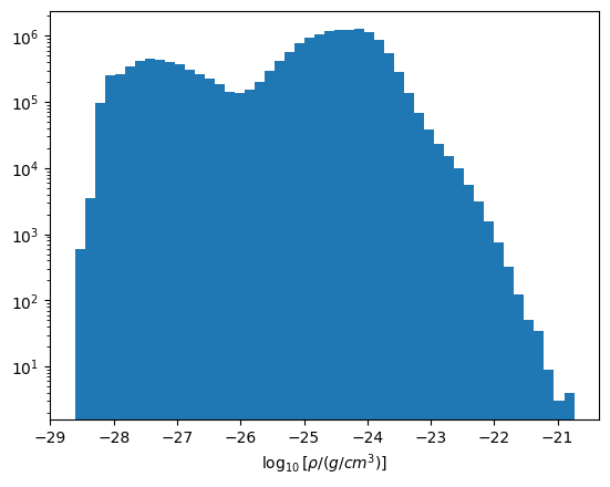
We can now look at, for example, the density distribution.
fig = plt.figure()
ax = fig.add_subplot(111)
ax.hist(np.log10(density_np.reshape(-1)), bins=50)
ax.set_yscale("log")
ax.set_xlabel(r"$\log_{10}[\rho / (g/cm^3)]$")
Use YT to analyse data#
The “ytds” member is the standard yt data object. You can use all the standard YT function to plot and analyse the data.
Below is a vertical slice of the gas density. You can see that this set of simulation data release contains only the galactic mid-plane region.
yt.SlicePlot(model.MHD.ytds, "x", ("gas", "density"))
