Synthetic dust polarization map#
import matplotlib.pyplot as plt
import numpy as np
Reading data (assuming that you’ve already downloaded the relevant data)#
# add path to astro_tigress module
# this can also be done using PYTHONPATH environment variable
import sys

sys.path.insert(0, "../")

import astro_tigress

# Need to set the master directory where the data is stored
dir_master = "../data/"
# name of the simulation model
model_id = "R8_4pc"
model = astro_tigress.Model(model_id, dir_master)  # reading the model information
# load the MHD data set for the snapshot ivtk=300
model.load(300, dataset="MHD")
Let’s convert the YT covering grid into numpy arrray with appropriate units. Magnetic fields are in microG. In the dust polarization map construction, only the ratio of different B components matters so that the units are not important for now. Also, I take transpose so that the array is in the original C-like ordering (z,y,x)
Temp = model.MHD.grid[("gas", "temperature")].in_units("K").value.T
nH = model.MHD.grid[("gas", "nH")].in_units("cm**-3").value.T
Bx = model.MHD.grid[("gas", "magnetic_field_x")].in_units("uG").value.T
By = model.MHD.grid[("gas", "magnetic_field_y")].in_units("uG").value.T
Bz = model.MHD.grid[("gas", "magnetic_field_z")].in_units("uG").value.T
Retrieve cell-centered coordinates for later uses.
xcc = model.MHD.grid[("gas", "x")][:, 0, 0].to("pc").value
ycc = model.MHD.grid[("gas", "y")][0, :, 0].to("pc").value
zcc = model.MHD.grid[("gas", "z")][0, 0, :].to("pc").value
Get cell size in pc and cm for convenience (note that the cell is cubic)
dx_pc = model.MHD.grid[("gas", "dx")][0, 0, 0].to("pc").value
dx_cm = model.MHD.grid[("gas", "dx")][0, 0, 0].to("cm").value
from astro_tigress.synthetic_dustpol import calc_IQU
I, Q, U = calc_IQU(nH, Bx, By, Bz, dx_pc, los="y")
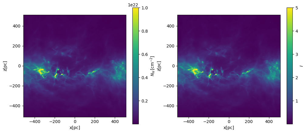
Projected column density and I#
fig, axes = plt.subplots(1, 2, figsize=(12, 5))
# integration along the y-axis (edge on view)
plt.sca(axes[0])
NH = nH.sum(axis=1) * dx_cm

plt.pcolormesh(xcc, zcc, NH, vmax=1.0e22, shading="nearest")
plt.gca().set_aspect("equal")
plt.xlabel("x[pc]")
plt.ylabel("z[pc]")
cbar = plt.colorbar(label=r"$N_H\,[{\rm cm^{-2}}]$")

plt.sca(axes[1])

plt.pcolormesh(xcc, zcc, I, vmax=5, shading="nearest")
plt.gca().set_aspect("equal")
plt.xlabel("x[pc]")
plt.ylabel("z[pc]")
cbar = plt.colorbar(label=r"$I$")
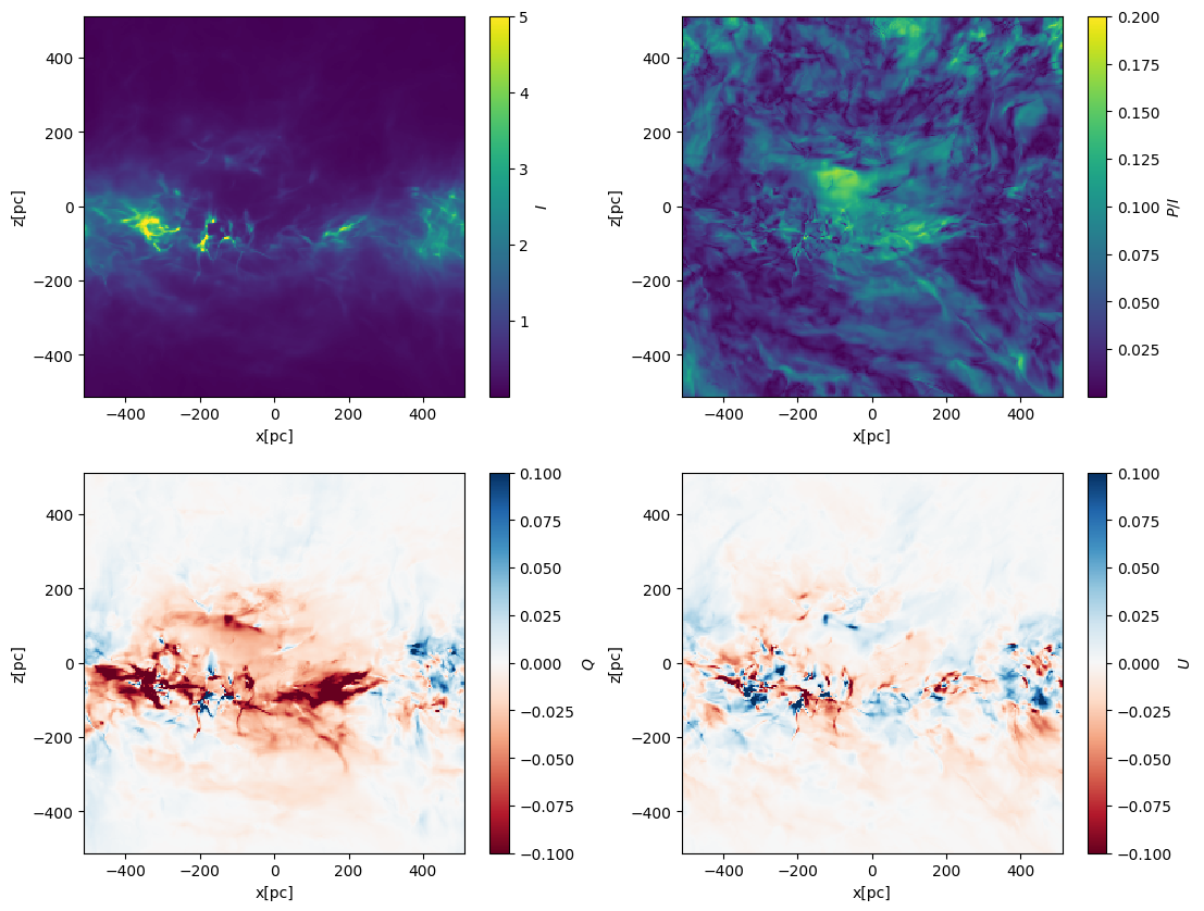
Polarization fraction, Q, and U maps#
P = np.sqrt(Q**2 + U**2)
fig, axes = plt.subplots(2, 2, figsize=(13, 10))
axes = axes.flatten()
# integration along the y-axis (edge on view)
plt.sca(axes[0])
plt.pcolormesh(xcc, zcc, I, vmax=5, shading="nearest")
plt.gca().set_aspect("equal")
plt.xlabel("x[pc]")
plt.ylabel("z[pc]")
cbar = plt.colorbar(label=r"$I$")
plt.sca(axes[1])
plt.pcolormesh(xcc, zcc, P / I, vmax=0.2, shading="nearest")
plt.gca().set_aspect("equal")
plt.xlabel("x[pc]")
plt.ylabel("z[pc]")
cbar = plt.colorbar(label=r"$P/I$")

plt.sca(axes[2])
plt.pcolormesh(xcc, zcc, Q, vmin=-0.1, vmax=0.1, shading="nearest", cmap=plt.cm.RdBu)
plt.gca().set_aspect("equal")
plt.xlabel("x[pc]")
plt.ylabel("z[pc]")
cbar = plt.colorbar(label=r"$Q$")
plt.sca(axes[3])
plt.pcolormesh(xcc, zcc, U, vmin=-0.1, vmax=0.1, shading="nearest", cmap=plt.cm.RdBu)
plt.gca().set_aspect("equal")
plt.xlabel("x[pc]")
plt.ylabel("z[pc]")
cbar = plt.colorbar(label=r"$U$")