Particle downsampling

Weights

In Tristan-MP v2 particles, along with other parameters like coordinates and momenta, have weights. This quantity is stored similarly on a tile tile%weight(p) (it has a type of real). Likewise the weight can be passed to particle injection functions:

call injectParticleGlobally(s, x, y, z, u, v, w, weight = 123.0)
! or
call createParticle(s, xi, yi, zi, dx, dy, dz, u, v, w, weight = 123.0)

Notice that the weight, 123.0, is in the form of a floating point number. If the weight is not passed, by default a particle with weight of 1.0 is created.

Particle weights are taken into account when computing the densities and energy densities saved into the flds.tot.***** files. Weights are also saved as particle quantities, and can then be accessed from prtl.tot.*****:

step = 137  # specify the step
filename = 'prtl.tot.%05i' % step
particles = isolde.getParticles(filename)
weights = particles['1']['wei'] # <- weights are saved into `wei` hdf5 database

Both pair production routines (Monte-Carlo and binary) respect particle weights, and adjust accordingly, i.e. two photons with weights 10.7 and 1.2 will pair-produce as if there were 11 particles in total. Photons with weights less than 1 do not participate in pair production. For this reason it is a good idea to make sure there are few photons below 1 in the simulation.

Particle downsampling

We provide a particle downsampling (or merging) routine performed on every tile (for massless and chargeless particles) or on every cell (for massive/charged particles). We employ a variation of the algorithm described by Vranic + (2015) where multiple particles in the same momentum bin are being merged into two, conserving weights, energy and momentum components. For charged particles the undeposited currents are taken care of with an extra deposit step (hence the constraint with merging region of only one cell).

For a particular species (say, species #3) to be considered for downsampling one has to specify explicitly in the input file:

<particles>

  # ...
  dwn3          = 1             # enable/disable particle downsampling

The downsampling parameters, also specified in the input, are the following:

<downsampling>

  # particle downsampling (merging) parameters (`dwn` flag)
  interval      = 10            # interval between downsampling steps [1]
  start         = 1             # starting timestep [0]
  max_weight    = 100           # maximum weight of merging particles [1e2]

  cartesian_bins = 0            # cartesian or spherical momentum binning [0]
  energy_min    = 1e-1          # min energy of merged particle [1e-2]
  energy_max    = 1e1           # max energy of merged particle [1e2]
  int_weights   = 1             # enforce integer weights when merging [0]

  # if spherical binning
  angular_bins  = 5             # number of angular bins (theta/phi) [5]
  energy_bins   = 5             # number of log energy bins [5]
  log_e_bins    = 1             # log or linear energy bins [1]

  # if cartesian binning
  dynamic_bins  = 1             # take min/max energy locally in each tile...
                                # (energ_max/min still set the global maxima) [0]
  mom_bins      = 5             # number of momentum bins in XYZ phase space [5]
  mom_spread    = 0.1           # max momentum spread allowed for dynamic bins [0.1]

Parameter int_weights makes sure that the resulting particles during downsampling have integer weights. For example, if the sum of all weights in a given momentum bin is 123 – two of the particles that others are merged into will have weights: 61 and 62 (otherwise, they would both have weights 61.5).

Warning: Downsampling may significantly reduce the memory usage and computation time depending on a given setup.

Warning: Downsampling also has some side effects. While it conserves the total weight, energy and momenta, and also properly mimics the (non-)uniformity in the phase space, downsampling routine alters the 3d distribution function by smoothing and flattening it. Depending on the application, this side-effect may be important, so consider change the energy ranges of merging particles or the number of bins.

There are two options for momentum binning: cartesian, where we bin separately all the components of particle momenta, and spherical.

Spherical binning

In this case (cartesian_bins = 0) the momentum binning is either logarithmic (log-normal) or linear in energy (specified by the log_e_bins parameter in the input file) and uniform in two spherical angles, similar to the method described for the Smilei code.

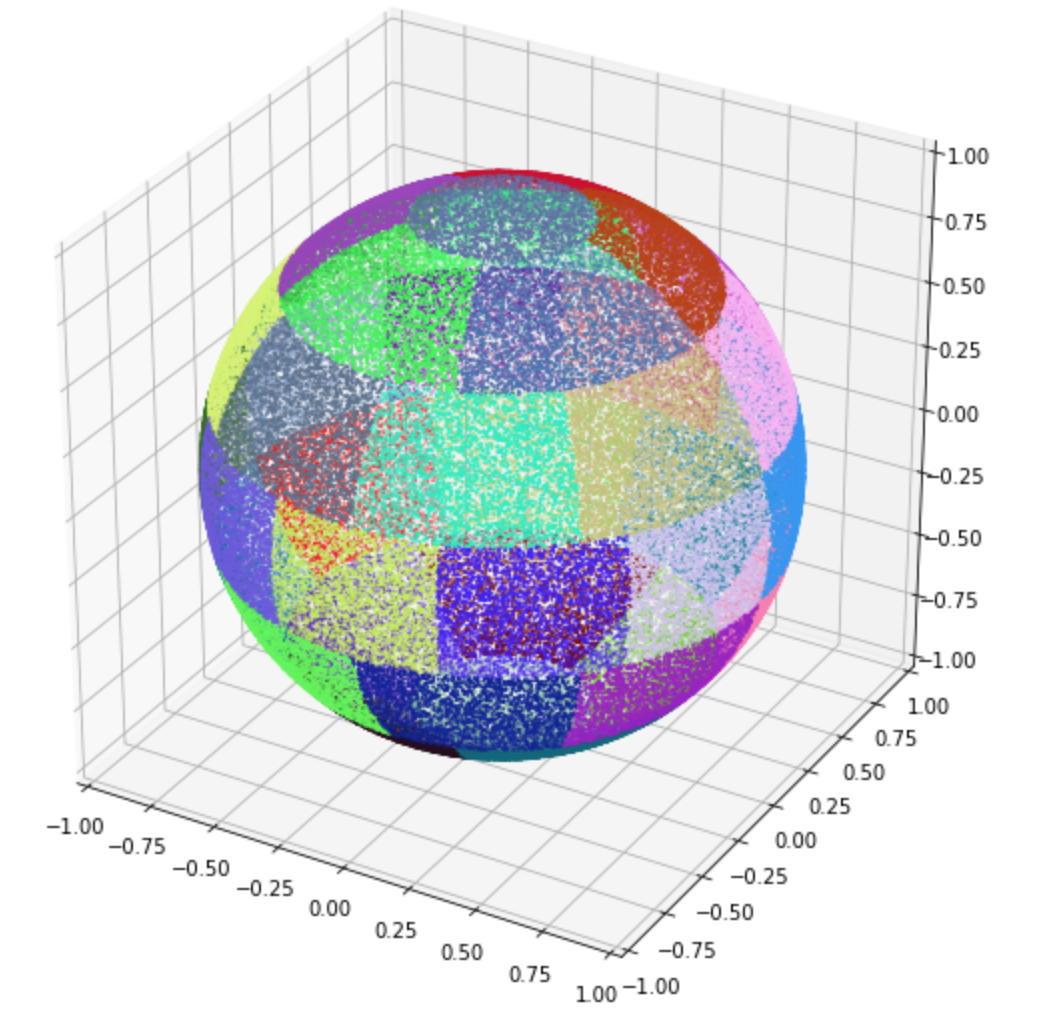
In the image above there are 100000 particles with equal energies scattered in the 3d phase space (unit sphere). Here we highlight groups of particles in the corresponding momentum bins with separate colors. At each timestep on every tile we also randomly rotate our momentum bins in 3d phase space, so that the two polar bins are not necessarily in $\pm z$ direction. The resulting merged population (in the same phase space) looks like the following:

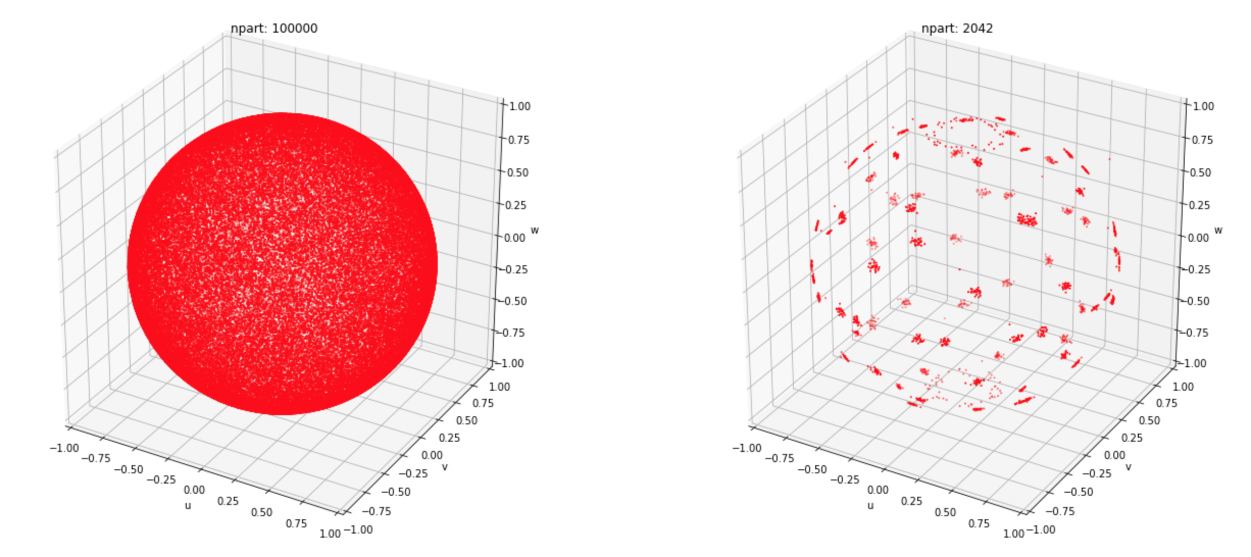
While now there are about 50 times less macro-particles (compare left and right panels), sum of all weights, energies and momentum components are precisely conserved.

Note: When specifying angular_bins = 5 there will actually be 5 + 2 = 7 bins in $\theta\in \left[-\pi/2, \pi/2\right]$ (with 2 additional polar bins), and 10 bins in $\phi \in \left[0, 2\pi\right]$.

Cartesian binning

When cartesian_bins = 1 is set in the input, all 3 components of the momenta are treated separately: the 3d phase space is separated into cubes. If the bins are static (dynamic_bins = 0), only the part of the phase space from $p_{x,y,z} \in [-p_{\rm max}, p_{\rm max})$ will be selected (other particles will be simply ignored). The value of $p_{\rm max}$ here is determined by the energy_max specified in the input.

Note: Keep in mind, that still only the particles with energy_min <= energy < energy_max will be participating in the downsampling.

If dynamic_bins = 1, the upper and lower boundaries of momentum bins will be dynamic: for each tile the code will precompute $p_{x,y,z}^{\rm min}$, $p_{x,y,z}^{\rm max}$ and $\langle p_{x,y,z} \rangle$. From this the lower and upper boundaries of the binned 3d phase space will be determined: pi_min = MAX(pi_min, pi_mid - 0.5 * mom_spread) and pi_max = MIN(pi_max, pi_mid + 0.5 * mom_spread). This method ensured that the binning is centered near the average momentum in a given tile (useful if there is a bulk flow), and that the size of the bin in each direction cannot exceed the mom_spread value defined in the input).