Visualization

Visualization

At the moment there are two ways to visualize the output data.

VisIt app

If hdf5 flag is enabled during the execution, along with the field quantities the code will also output the .xdmf files. These are basically xml formatted files that contain the detailed description of the data structure in the flds.tot.***** (see details here). This is necessary for the VisIt visualization app to recognize the hdf-files and be able to read them. VisIt is probably the fastest way to visualize three dimensional field quantities. You can enable/disable the output of these auxiliary files from the input file:

<output>
  # ...
  write_xdmf    = 1              # enable XDMF file writing (to open hdf5 in VisIt)
  # ...

python module

As every Tristan in legends and stories come with his Iseult, our Tristan also has it’s own isolde which is a data reading and visualization package for python. The usage is fairly simple. We will first need to import the module by doing

import tristanVis.isolde as isolde

Read particles

step = 137  # specify the step
filename = 'prtl.tot.%05i'%step
particles = isolde.getParticles(filename)

particles is now a nested dictionary containing all the particle species and their relevant saved quantities:

electrons = particles['1']    # take all the electrons
electrons_x = electrons['x']  # take all the x-positions of the electrons
print (electrons.keys())      # enumerate all the saved quantities

Read fields

step = 137  # specify the step
filename = 'flds.tot.%05d'%step
fields = isolde.getFields(filename)

fields is now a dictionary of three dimensional arrays with all the relevant fields saved. By default they are:

print (fields.keys())
# ['xx', 'yy', 'zz', 'ex', 'ey', 'ez', 'bx', 'by', 'bz', 'jx', 'jy', 'jz', 'dens1', 'dens2', ...]
# 3d grid points, ...
# ... electric field components, ...
# ... magnetic field components, ...
# ... current density components and ...
# ... the densities of all the species

fields['xx'], if you are familiar with numpy terminology is the meshgrid – all the corresponding x coordinates of the domain in a 3d array.

Read spectra

The following is to read the distribution functions for all the particle species.

step = 137  # specify the step
filename = 'spec.tot.%05d' % step
spectra = isolde.getSpectra(filename)

spectra is now an instance of custom class Spectra that contains all the information we need (remember, the spectra are saved binned both in energy and in space). For instance, we can see the energy bins (common for all the species) with spectra.ebins, and spatial bins in x direction with spectra.xbins. We can access the total spectrum of species #1 summed over all the spatial bins by doing spectra.getTotal(1). We can also access the information for a given species in a given spatial bin either by coordinate (in code units) or the bin index: spectra.getByCoordinate(1, (123.5, 56.3, 0.3)) or spectra.getBySpatialBin(1, (5, 12, 0)).

Read domain distribution

Tristan also saves the domain distribution data, i.e., how the simulation box is subdivided between the MPI processes.

step = 137  # specify the step
filename = 'domain.%05d'%step
domains = isolde.getDomains(filename)

Now domains will contain a dictionary with the sizes (sx, sy, sz) and the coordinates of the “left bottom” corners of the MPI domains (x0, y0, z0).

Parse the report, history and input files

History output can be parsed using the predefined function in the isolde module:

import tristanVis.isolde as isolde
hist_data = isolde.parseHistory('history')

The report file contains crucial information about the performance capabilities of your run, including the data on how long each of the loop substeps take, how different are the loads on each MPI process and how many particles of each species do we host on each core. To make life easier, isolde provides a very useful function to parse this report file and save all the interesting quantities to a dictionary.

interval = 10       # parse every 10-th step
num_steps = 100500  # how many steps to parse
filename = 'report' # specify the location of the `report` file
report = isolde.parseReport(filename, nsteps = num_steps, skip = interval)

report is now a dictionary with the following keys:

print (report.keys())
# ['t', 'Full_step', 'move_step', 'deposit_step', ..., 'output_step', 'nprt 1 [core]', 'nprt 2 [core]', ...]
# 't' - timestep
# 'Full_step' - duration of the whole step
# 'nprt 1 [core]' - average number of particles per core of the species 1

For each of these step/substep durations we can find the mean duration dt, and the min and max durations among the MPI processes to estimate the possible load imbalance.

In the same way one can parse the input file to obtain the relevant quantities specified at the runtime:

import tristanVis.isolde as isolde
input_params = isolde.parseInput(input_file_name)

Now the input_params is a depth-2 dictionary with all the parameters. To obtain, say, the speed of light specified one would do:

input_params['algorithm']['c']
# in general: input_params[<BLOCKNAME>][<VARIABLE>]

Built-in visualization functions

There are a couple of very useful python scripts that are included with this code to help make analysis of data and interaction with it much easier. First of all there are three libraries that you might want to preload to access these capabilities:

import tristanVis.tristanVis as tVis
import tristanVis.snippets as trS
import tristanVis.isolde as isolde
trS.loadCustomStyles(style='default', fs=15)

The last line will enable LaTeX with matplotlib, load several colormaps (e.g. fire and bipolar) which are unavailable in standard matplotlib, and configure a few settings with the font. You can pass any style supported by matplotlib (e.g. dark_background, fivethirtyeight).

Loading field data for the whole simulation

To load a field data for certain timesteps from a simulation output directory you may use the following function:

# if `fld_steps` is not specified it loads all the available timesteps
sim = tVis.Simulation('/path/to/output/', fld_steps=np.arange(0, 50, 5))
sim.loadData() # < this call actually loads everything into memory

Now you can access your data at timestep 5 by: sim.fields[5].data['z=0'] which is an xarray dataset with all the fields in corresponding coordinates. The subscript ['z=0'] simply means this is a 2d simulation, otherwise this could have been a slice from 3d simulation, in which case you would have used tVis.Simulation(..., useSlices=True) (it would have loaded all the available slices).

Before doing sim.loadData() you can actually add additional secondary variables you want to keep in memory, or, say, make a coordinate transformation:

# define an E.B variable
sim.addVariables({'e.b': lambda f: (f['ex']*f['bx'] + f['ey']*f['by'] + f['ez']*f['bz'])})
# transform coordinates dividing them by skin depth (defined as `c_omp` somewhere else)
sim.addCoordinateTransformation({'x': lambda x: x / c_omp,
                                 'y': lambda y: y / c_omp,
                                 'z': lambda z: z / c_omp})
# mask data
sim.maskData(lambda f: f['e.b'] > 0.1)
# now load everything
sim.loadData()

Now when you load the data it will contain these new variables, the coordinates are going to be properly scaled and the data will be masked according to rule you prescribed. xarray allows to easily display the 2d data by doing sim.fields[5].data['z=0']['e.b'].plot().

Interactive plotting

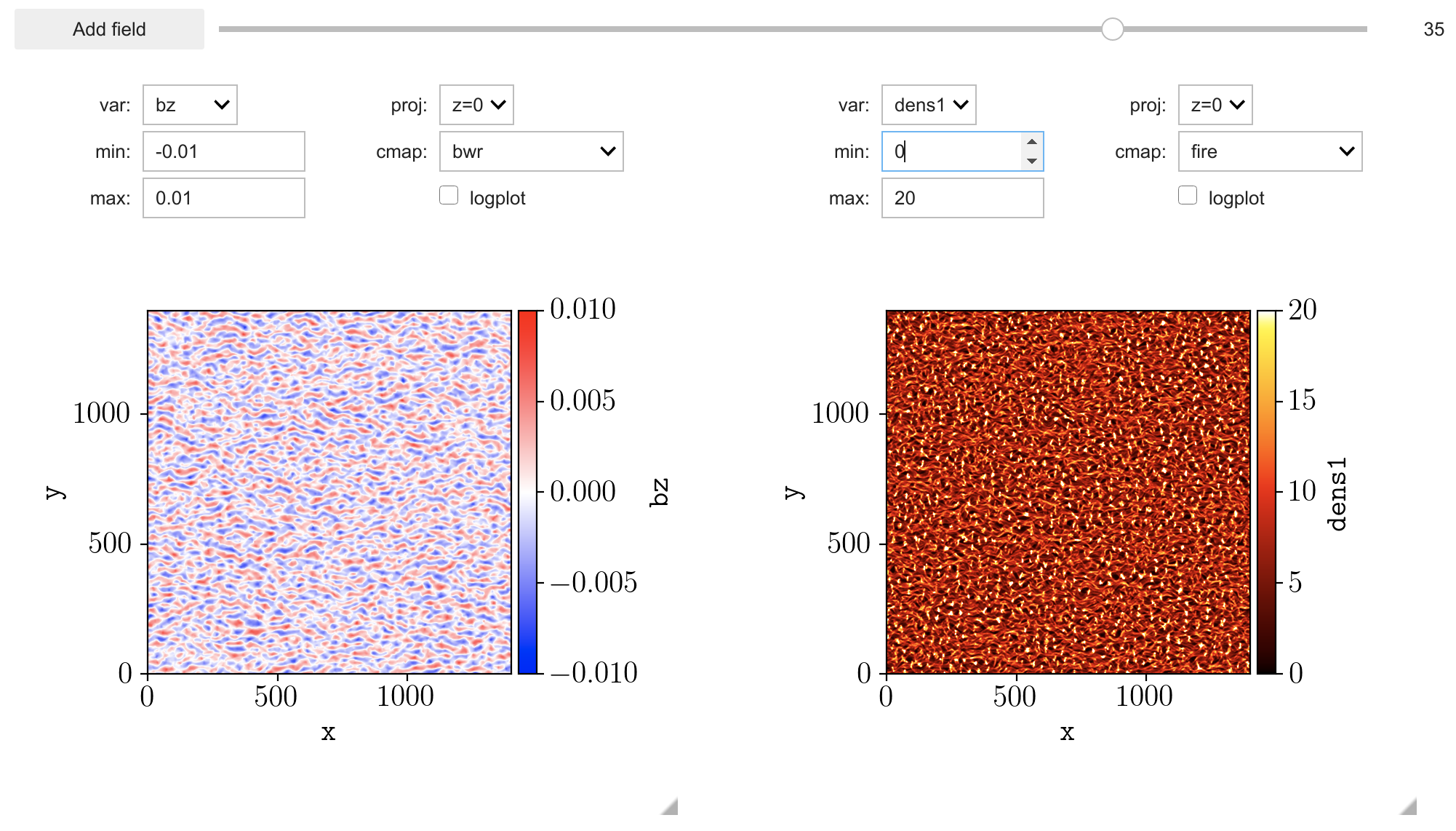
If you’re using jupyter – there are even more capabilities you can employ. You can use the interactive field plotting routine to go over the timesteps of your simulation, configure colorbars and scalings, etc. To do that simply run the following two lines in your jupyter (make sure you’re in the %matplotlib widget regime):

grid = tVis.PlotGrid(sim, controls=True, figsize=(4.5, 4))
grid.show()

This will open a window similar to the following where you can add as many panels as you like with the field variables plotted in 2d, change colormaps and min/max values and swipe through the timesteps.

If you want to save the state (configurations) to reuse later – you may do so by running grid.exportParameters('myfile.json'). Then when you want to load the state again, you run:

grid = tVis.PlotGrid(sim, controls=True, figsize=(4.5, 4))
grid.readParameters(filename='myfile.json')
grid.show()

If you want to save current panels as a png file, you can run grid.savePng('myimage.png').