Load balancing is a way to distribute the computational domain between MPI processes in such a way, that all processes have roughly the same computational load (e.g., number of particles per core). There are two basic approaches: static and dynamic (adaptive). In the first case, we split the simulation domain and assign the resulting meshblocks to the MPI processes in the very beginning (according to a certain user defined function), and we never change the meshblock dimensions and distributions any time in the future. In the adaptive case we do this redistribution routine once every few timesteps.
Static load balancing
Static load balancing for Tristan-MP v2 has to be turned on during the configuration with -slb flag. When we do that, we should see the following line:
Load balancing: static
In the input file we also need to specify the corresponding parameters under the <static_load_balancing> block (check the input.dummy file):
<static_load_balancing>

  in_x         = 1
  sx_min       = 10

  in_y         = 1
  sy_min       = 10

  in_z         = 0
  sz_min       = 10
Here in_x, in_y, in_z are either 1 or 0 to turn the static load balancing ON and OFF in the corresponding direction. And s*_min is the minimum number of cells (in one dimension) that an MPI domain can have during a redistribution in the corresponding dimension (having less than a few cells in any direction is inefficient).
Now we also need to specify the function according to which the load should be balanced at the very beginning (before particle initialization etc). This is done in the user file, where we define a function pointer user_slb_load_ptr which points at the userSLBload() function (also defined in the user file, see unit_slb.F90 for an example).
This userSLBload() takes 3 + 3 arguments (global coordinates of the cell and three spatial dimensions of the global simulation box) and returns the weight of the given cell: the higher the weight, the more time an MPI process will spend computing that cell. Meaning, our SLB routine will try to assign more MPI processes to the regions with high weights. This weight, of course, is an abstract value for each cell, and has no physical significance on its own. It’s only intention is to be used to balance the loads once at the very beginning of the simulation.
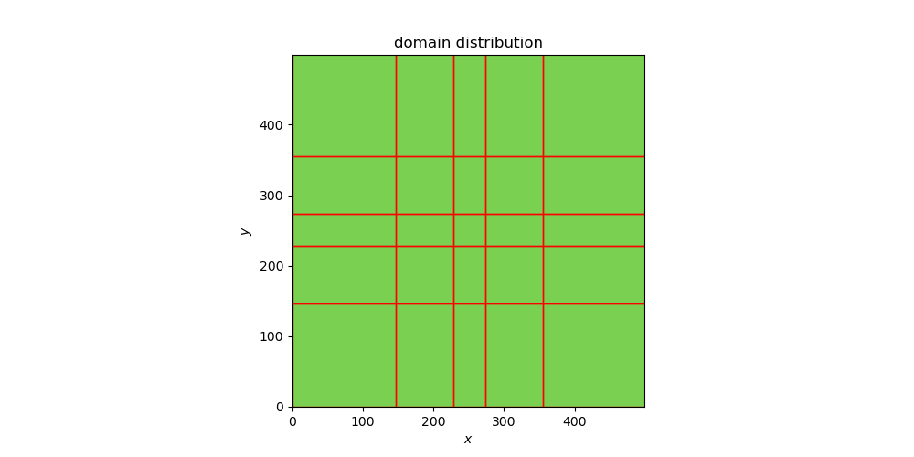
As an example, we can use a centrally clumped spatial distribution (e.g., if we’re simulating a neutron star with a lot of particles in the middle of the box):
 function userSLBload(x_glob, y_glob, z_glob,&
                      & dummy1, dummy2, dummy3)
   real :: userSLBload
   ! global coordinates
   real, intent(in), optional  :: x_glob, y_glob, z_glob
   ! global box dimensions
   real, intent(in), optional  :: dummy1, dummy2, dummy3
   real                        :: radius
   radius = sqrt((dummy1 * 0.5 - x_glob)**2 + (dummy2 * 0.5 - y_glob)**2) + 1.0
   userSLBload = 10.0 / radius
   return
 end function
which results in the following distribution of meshblocks.
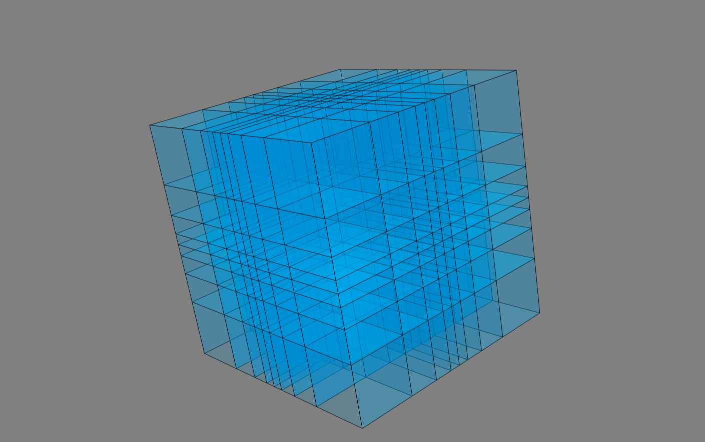
Below is another example of static load balancing done in three dimensions with meshblocks concentrated at the center of the grid.
Adaptive load balancing
Since version v2.2 adaptive load balancing during runtime is also supported. It is enabled with the -alb flag during the code configuration. Adaptive load balancing has the following configurations that can be set from the input file (their explanations as well as default values are shown below).
<adaptive_load_balancing>

  # (if `alb` flag is enabled)
  in_x         = 1               # enable along x [0]
  sx_min       = 10              # min # of cells per meshblock [10]
  interval_x   = 100             # timesteps between load balancing in x [1000]
  start_x      = 1000            # first timestep for load balancing in x [1]
  slab_x       = 10              # slab to be sent in x direction [1]

  in_y         = 1               # enable along y [0]
  sy_min       = 10              # min # of cells per meshblock [10]
  interval_y   = 100             # timesteps between load balancing in y [1000]
  start_y      = 1000            # first timestep for load balancing in y [1]
  slab_y       = 10              # slab to be sent in y direction [1]

  in_z         = 1               # enable along z [0]
  sz_min       = 10              # min # of cells per meshblock [10]
  interval_z   = 100             # timesteps between load balancing in z [1000]
  start_z      = 1000            # first timestep for load balancing in z [1]
  slab_z       = 10              # slab to be sent in z direction [1]