Writing a user file | Tristan v2

In this section we are going to learn the basics of writing a user file in Tristan-MP v2.

As an example we are going to write a user file for a two dimensional double periodic reconnection setup, since it involves some of the most basic and necessary routines and building blocks.

Start by copying and renaming the default user/user_dummy.F90 (to, say, user/user_myrec.F90) as it contains the most up-to-date default routines for initialization that we’ll need to be filling in.

Reading input parameters

First we will need to read the setup parameters from the input file and store them in some local variables. For that we can use the getInput() routine inside of the userReadInput(). There you need to specify the block (<problem>), the variable name and the variable itself (we will declare them later). This is what the code looks like.

subroutine userReadInput()
  implicit none
  call getInput('problem', 'upstream_T', upstream_T)      ! <- upstream temperature
  call getInput('problem', 'nCS_nUP', nCS_over_nUP)       ! <- density of the current sheet / density upstream
  call getInput('problem', 'current_width', current_width)
  cs_x1 = 0.25; cs_x2 = 0.75 ! <- positions of current sheets (as a fraction of the global size)
end subroutine userReadInput

Note: There is no need to specify the variable type (real/integer/logical), as the function getInput will do the necessary conversion itself, given the type from the variable declaration (see below).

Also don’t forget to declare all these variables in the top:

!--- PRIVATE variables -----------------------------------------!
real :: upstream_T, current_width, cs_x1, cs_x2, nCS_over_nUP
private :: upstream_T, current_width, cs_x1, cs_x2, nCS_over_nUP
!...............................................................!

Note: making them private is optional and is primarily for safety reasons.

To pass the desired values, we need to add the following block to the input file:

<problem>

  upstream_T      = 1e-5           # temperature in terms of [m_e c**2]
  nCS_nUP         = 3.0
  current_width   = 10

Initializing particles

After we are done with the variables, we can initialize the particles, which is done in the conveniently named userInitParticles() routine. First we’ll need to declare a few variables:

real            :: nUP, nCS
type(region)    :: fill_region
real            :: sx_glob, sy_glob, shift_gamma, shift_beta, current_sheet_T
procedure (spatialDistribution), pointer :: spat_distr_ptr => null()
spat_distr_ptr => userSpatialDistribution

The last two lines are from the user_dummy.F90, they are to specify the spatial distribution function of injected plasma. Let us leave them aside for now and get back to them later.

After we’ve declared these variables we can define the upstream and current sheet densities as well as the initial temperature and the current density of the current sheets, necessary to balance the curl B and B^2 (the following is for the electron-positron plasma).

nUP = 0.5 * ppc0
nCS = nUP * nCS_over_nUP

! initial drift velocity of the current sheet
!     to ensure `curlB = j`
shift_beta = sqrt(sigma) * c_omp / (current_width * nCS_over_nUP)
if (shift_beta .gt. 1) then
  ! making sure `beta < 1`
  call throwError('ERROR: `shift_beta` > 1 in `userInitParticles()`') ! < this will stop simulation with an error
end if
shift_gamma = 1.0 / sqrt(1.0 - shift_beta**2)
!     to ensure `B^2/2 = sigma T n me c^2`
current_sheet_T = 0.5 * sigma / nCS_over_nUP

Notice the fill_region variable of type (region) declared above. That object basically defines a region (on a domain or meshblock) where the plasma will be sprinkled (i.e., we will be passing that variable to an injection routine). In this case we will be filling the entire domain, and will take care about spatial distribution function later. So for now, we will specify the entire domain as the dimensions of this region:

fill_region%x_min = REAL(0)
fill_region%y_min = REAL(0)
fill_region%x_max = REAL(global_mesh%sx)
fill_region%y_max = REAL(global_mesh%sy)

Tip: If you are unfamiliar with this_meshblock%ptr etc, take a look at this section.

After that we are ready to inject the upstream particles. For that we will need to call the fillRegionWithThermalPlasma() routine and pass the following variables:

the filling region, fill_region;
all the species as an array, in this case it’s just /(1, 2)/;
the number of species passed, i.e., length of the array above, in this case – 2;
initialization density for all of the species;
the temperature.

The upstream plasma is sprinkled everywhere and with the zero drift, so we don’t need to specify anything else. For the current sheet, however, we will need to specify a few other things:

drift velocity – Lorentz factor of the boosted Maxwellian, shift_gamma;
direction of the boost (+/-1 = +/-x, +/-2 = +/-y, +/-3 = +/-z): by default positively charged particles are boosted in the direction specified, negatively charged ones – in the opposite direction;
pointer to the predefined spatial distribution function, spat_distr_ptr;
a few variables to pass to the spatial distribution function (if necessary).

Here’s what the injection looks like:

sx_glob = REAL(global_mesh%sx) ! <- define global simulation size in `x`

! now filling region with plasma
!     upstream:
call fillRegionWithThermalPlasma(fill_region, (/1, 2/), 2, nUP, upstream_T)
!     current sheet #1:
!       positrons fly in +z
call fillRegionWithThermalPlasma(fill_region, (/1, 2/), 2, nCS, current_sheet_T,&
                               & shift_gamma = shift_gamma, shift_dir = 3,&
                               & spat_distr_ptr = spat_distr_ptr,&
                               & dummy1 = cs_x1 * sx_glob, dummy2 = current_width)
!     current sheet #2:
!       positrons fly in -z
call fillRegionWithThermalPlasma(fill_region, (/1, 2/), 2, nCS, current_sheet_T,&
                               & shift_gamma = shift_gamma, shift_dir = -3,&
                               & spat_distr_ptr = spat_distr_ptr,&
                               & dummy1 = cs_x2 * sx_glob, dummy2 = current_width)

fillRegionWithThermalPlasma creates particles of specified species (positioned at the same location) with a specified density, temperature and boost. dummy1 and dummy2 are the two optional parameters, in this case the position and the width of the current sheet, passed to the spatial distribution function.

The latter needs to be also defined in the user file. Notice that spat_distr_ptr in the declaration above is at the moment pointing at a function userSpatialDistribution() also defined in the user file. That userSpatialDistribution() is basically a “wave function” for the particle, that returns a probability to inject a particle in a particular location x_glob, y_glob, z_glob. Let us define it in such a way that it injects particles primarily around our current sheets. Since we will be using the tanh profile for the b-field, we’ll need to use 1/cosh^2 for the density, so we can simply change the “wave function” to the following:

function userSpatialDistribution(x_glob, y_glob, z_glob,&
                               & dummy1, dummy2, dummy3)
  real :: userSpatialDistribution
  real, intent(in), optional  :: x_glob, y_glob, z_glob
  real, intent(in), optional  :: dummy1, dummy2, dummy3
  ! dummy1 -> position of the current sheet
  ! dummy2 -> width of the current sheet
  userSpatialDistribution = 1.0 / (cosh((x_glob - dummy1) / dummy2))**2
  return
end function

Tip: detailed description of particle structure can be found here.

Initializing fields

Field initialization is fairly straightforward, except that we need to worry about the staggering. In this case we will only be initializing the by as a function of x, so we don’t have to worry about staggering at all. Here is what the userInitFields() routine should look like:

subroutine userInitFields()
  implicit none
  integer :: i, j, k
  real    :: sx_glob, x_glob
  ! initializing everything to zero
  ex(:,:,:) = 0; ey(:,:,:) = 0; ez(:,:,:) = 0
  bx(:,:,:) = 0; by(:,:,:) = 0; bz(:,:,:) = 0
  jx(:,:,:) = 0; jy(:,:,:) = 0; jz(:,:,:) = 0

  sx_glob = REAL(global_mesh%sx)
  ! loop through all the cells
  do i = 0, this_meshblock%ptr%sx - 1
    ! converting to global (explicit conversion is optional)
    x_glob = REAL(i + this_meshblock%ptr%x0)
    do j = 0, this_meshblock%ptr%sy - 1
      do k = 0, this_meshblock%ptr%sz - 1
        ! no staggering in this case
        by(i, j, k) = tanh((x_glob - cs_x1 * sx_glob) / current_width) -&
                    & tanh((x_glob - cs_x2 * sx_glob) / current_width) - 1
      end do
    end do
  end do
end subroutine userInitFields

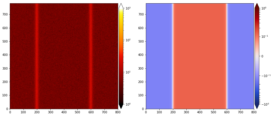
Tip: For details about the fields see here.

And that’s it. If you run it and read the initial data, it will produce something similar to this (left panel: density, right panel: by):

Tip: To learn how to read the output and visualize the data, please read the following chapter.