Memory structure
There are three main objects which are stored in memory locally on every core.
1. Simulation domain and its decomposition.
Each core has the information about the whole simulation domain and its decomposition, meaning that every MPI unit (core) knows which part of the domain is assigned to all the other MPI units. All the relevant information is stored locally in the meshblocks(:) array, which has a size of mpi_size (number of MPI processes launched).
2. Fields in the cells of the local subdomain.
Field quantities, such as the components of the electric and magnetic field, as well as the components of the current density are stored locally on each MPI unit. These are simple 3d arrays for the cells corresponding to specific subdomain assigned to the specific MPI rank. These field arrays are, however, slightly larger than the size of the local subdomain (by NGHOST cells in each dimension) which allows to store a small part of data from the neighboring subdomains. This vastly increases the performance by decreasing the number of MPI communications required.
3. Particles.
Since Tristan-MP v2 is has a multi-species architecture, particles are stored in the array called species(:). Each species(s) object has a three dimensional array of tiles, prtl_tile(:,:,:), which basically subdivides the local subdomain into finer regions (typically few cells in size). These tiles further contain all the necessary particle information, such as coordinates and velocities.
Visually the structure looks like the animation below. Further in this section we will discuss all the components in more details.
Domains
src/objects/domain.F90.MPI Parallelism
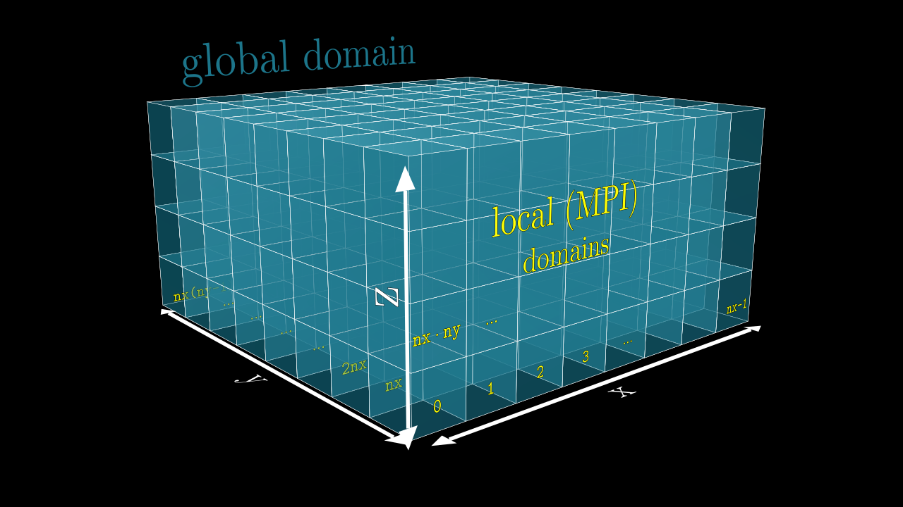
The key concept here is the meshblock or MPI domain (unit). Every core on the cluster is responsible for the computation on a certain chunk of the global domain. Let’s say we have a global simulation domain consisting of mx * my * mz cells in all 3 directions, and let’s assume we have N = nx * ny * nz cores. Given that mx, my and mz are divisible by nx, ny and nz, we can distribute our global simulation domain evenly between all N cores, each core doing computation on a particular grid of the size (mx/nx) * (my/ny) * (mz/nz).
The illustration of this is shown in the image below, red numbers on each meshblock is the corresponding MPI rank, rank of the core which operates on a given domain. Notice how the ranking goes from 0 to nx - 1 along x-axis, etc, the last rank will be the nx * ny * nz - 1.
During our simulation we will need to interchange information between the MPI processes (e.g., send field quantities back and forth, send particles, etc), and for that we will need to know exactly what the neighborhood of our current MPI meshblock is (i.e., what MPI rank operates there etc).
Meshblocks (MPI Domains)
All MPI processes perform the same code on a chunk of the global domain corresponding to their rank. In order to keep these processes synced, we keep track of how the entire (global) simulation domain is distributed between the MPI processes. For that we have the fortran type called mesh. We keep track of all meshblocks in an array of type mesh:
type(mesh) :: meshblocks(MPI_size)
! (i-1)-st rank operates on `meshblocks(i)`, where i goes from `1` to `MPI_size`
meshblocks(i)%sx  ! <- # of cells in x direction for the i-th meshblock
meshblocks(i)%sy  ! <- # of cells in y direction
meshblocks(i)%sz  ! <- # of cells in z direction
meshblocks(i)%x0  ! <- global x-coordinate of the meshblock's corner in the global domain
meshblocks(i)%y0  ! <- global y-coordinate of the meshblock's corner in the global domain
meshblocks(i)%z0  ! <- global z-coordinate of the meshblock's corner in the global domain
meshblocks(i)%rnk ! <- rank of the MPI process operating on this meshblock
meshblocks(i)%neighbor(:,:,:) ! <- array with pointers to all neighbors of this particular meshblock

Meshblock pointers
Every local MPI process “knows” about the global structure of the whole simulation domain (which MPI ranks are assigned to which meshblocks etc) through the meshblocks(:) array. To make life easier we also provide an auxiliary type to mesh, which is the meshptr – a pointer to a mesh-type object. For example, to get the current (local) mesh one can simply do:
this_meshblock%ptr    ! <- if we are on rank `i` this will return `meshblocks(i+1)`
this_meshblock%ptr%sx ! <- # of cells in x for current (local) meshblock
...
With the help of this construct one can also access the neighboring meshblocks and directly address them (e.g., communicate through MPI). The example is shown below.
! (i-1)-st MPI rank lives on `meshblocks(i)`
meshblocks(i)%neighbor(+1, 0, 0)%ptr ! <- `mesh`-type object of the direct neighbor in +x direction
meshblocks(i)%neighbor( 0,+1,-1)%ptr ! <- `mesh`-type object of the direct (diagonal) neighbor in +y/-z direction
this_meshblock%ptr%neighbor(+1,-1, 0)%ptr ! <- ... you got the point
...%ptr is a purely Fortran thing, fortran does NOT allow to have a pointer on an array element of the user-defined type. So we had to make a workaround.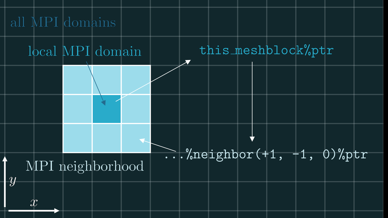
Example of usage
If a particle leaves the region our current domain is operating on we will have to send this particle to a new neighboring MPI domain. Let’s say a particle leaves through a upper (+z), left (-x) corner. We can easily verify this by checking the coordinates of our particle (this is just an example):
(prt_x .lt. 0) .and. (prt_z .ge. this_meshblock%ptr%sz) ! <- this will be `.true.`
This means our current MPI process will need to send this particle to an MPI process with rank:
this_mesblock%ptr%neighbor(-1, 0,+1)%ptr%rnk
Fields
src/objects/fields.F90.There are 9 basic field components: ex, ey, ez, bx, by, bz, jx, jy, jz. These objects are fairly straightforward: they are just 3 dimensional arrays containing the corresponding components of E-field, B-field and current densities. However there are a few things to keep in mind.
Indexing
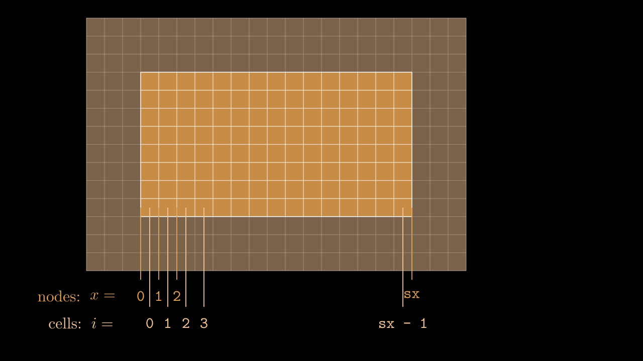
The numbering of cells in a given MPI domain in each direction goes from 0 to sx - 1 (remember, sx is our this_meshblock%ptr%sx). This means that field values in these cells will be stored in, say, ex(i, j, k) with i running from 0 to sx - 1, j is running from 0 to sy - 1, etc. Notice, that the real physical coordinates of these cells correspond not to cell centers, but to nodes (see image below).
Staggering
While real-life electric and magnetic field components are continuous and defined in each and every point in three-dimensional space, the values we store in our arrays are obviously discrete. To make life easier we exploit the so-called staggered, or Yee mesh for storing the electric and magnetic field components (see animation below). This means that a value ex(i, j, k) is not really a value of the real field in the center of the cell (i, j, k), but instead is a value on one of the edges as shown in the image below. So strictly speaking by writing ex(i, j, k) we really mean $e_x^{i,j-1/2,k-1/2}$. This logic applies to all the field components, including the current density components, which alike the electric field are also stored on the edges of the corresponding cell.
Ghost cells
During our simulation we might need to compute the field value in a particular spatial position (e.g., at the position of the particle) for which we would interpolate the corresponding component values to a given position. This means that at some point we might need to know a field value stored on a neighboring meshblock. To minimize communications between MPI domains we store some additional fields quantities from the neighboring meshblocks in the so-called ghost zones (denoted by red in the image below). Every timestep we update the values in these ghost cells so they contain the most up-to-date data on the field quantities of neighboring MPI domains.
Conveniently, the indexing of ghost zones (say, in x) goes like:
NGHOSTghost cells on the left:i = -NGHOST, ..., -1;sxactive cells:i = 0, ..., sx - 1;NGHOSTghost cells on the right:i = sx, ..., sx + NGHOST - 1.
Here NGHOST is a global variable defined on a compilation time which determines how many ghost zones we want to use in our simulation.
Usage example
Let’s say we want to setup an electromagnetic field propagating in xy direction in a periodic box. Here’s a simple loop that will do the job.
! `kx` and `ky` are the wavenumbers in global coordinates:
kx = 5; ky = 2
kx = kx * 2 * M_PI / global_mesh%sx
ky = ky * 2 * M_PI / global_mesh%sy

! normalizing the field components />
if (ky .ne. 0) then
  ex_norm = 1; ey_norm = (-kx / ky)
else
  ey_norm = 1; ex_norm = (-ky / kx)
end if
exy_norm = sqrt(ex_norm**2 + ey_norm**2)
ex_norm = ex_norm / exy_norm
ey_norm = ey_norm / exy_norm
! </ normalizing the field components

! loop through all the active cells of the current MPI domain
do i = 0, this_meshblock%ptr%sx - 1
  i_glob = i + this_meshblock%ptr%x0 ! <- converting local to global coordinates
  do j = 0, this_meshblock%ptr%sy - 1
    j_glob = j + this_meshblock%ptr%y0
    do k = 0, this_meshblock%ptr%sz - 1
      k_glob = k + this_meshblock%ptr%z0
      ! notice that `ex` is staggered in y and z direction ...
      ex(i, j, k) = ex_norm * sin((i_glob) * kx + (j_glob - 0.5) * ky)
      ! ... and `ey` is staggered in x and z direction ...
      ey(i, j, k) = ey_norm * sin((i_glob - 0.5) * kx + (j_glob) * ky)
      ez(i, j, k) = 0
      bx(i, j, k) = 0
      by(i, j, k) = 0
      ! ... and `bz` is staggered in z direction
      bz(i, j, k) = sin((i_glob) * kx + (j_glob) * ky)
    end do
  end do
end do
Particles
src/objects/particles.F90.Particles along with fields are the heart and soul of every particle-in-cell code. Particles sample the kinetic distribution function of the multicomponent plasma and also enable to track the dynamics of massless photons.
Species
In this code we support arbitrary number of species that are treated separately. To take care of that we have a special type called particle_species which has an instance array, species(:), containing all the information about particle species.
Structure of species type
The species(s) objects, where s = 1, ..., nspec, contain useful information about the particular particle species, as well as all the data about individual particles themselves. Let’s have a look at what this object contains:
| Attribute | Description | Default value if not specified | Used with flag… |
|---|---|---|---|
cntr_sp |
integer counter to keep track of indexing for the newly created particles | – | |
m_sp, ch_sp |
mass and charge (normalized to code units) | – | – |
tile_sx, tile_sy, tile_sz |
dimensions of particle tiles | – | – |
tile_nx, tile_ny, tile_nz |
numbers of particle tiles | – | – |
deposit_sp |
do particles deposit | .true. if ch_sp != 0 |
– |
move_sp |
do particles move | .true. |
– |
output_sp |
are particles saved into the prtl.tot. file |
.true. |
– |
cool_sp |
are particles cooled | .true. if ch_sp != 0 |
--radiation |
dwn_sp |
can particles be downsampled (merged) | .false. |
-dwn |
bw_sp |
0 means species does not participate in BW process, 1 and 2 would be separate BW groups |
0 |
-bwpp |
compton_sp |
do particles participate in Compton scattering | .false. |
-compton |
gca_sp |
can particles be treated in the GCA approach | .true. if ch_sp != 0 |
-gca |
Along with all the common information, the object species(s) also contains the individual particles themselves which exist on the so-called tiles (species(s)%prtl_tile(:,:,:)%...).
Tiles and particles
Tiles are basically smaller chunks of the MPI domain (contained locally within a single MPI process) which store all the information about the particles (see image below).
Their dimension can be configured from the input file, and their number in each direction depends on the local domain size and the size of each individual tile (notice, that some of them might be smaller than ...%tile_sx/sy/sz. Left and right (up/down, front/back) boundaries of the tile are stored on it as well ...%prtl_tile(ti, tj, tk)%x1/x2/y1/y2/....
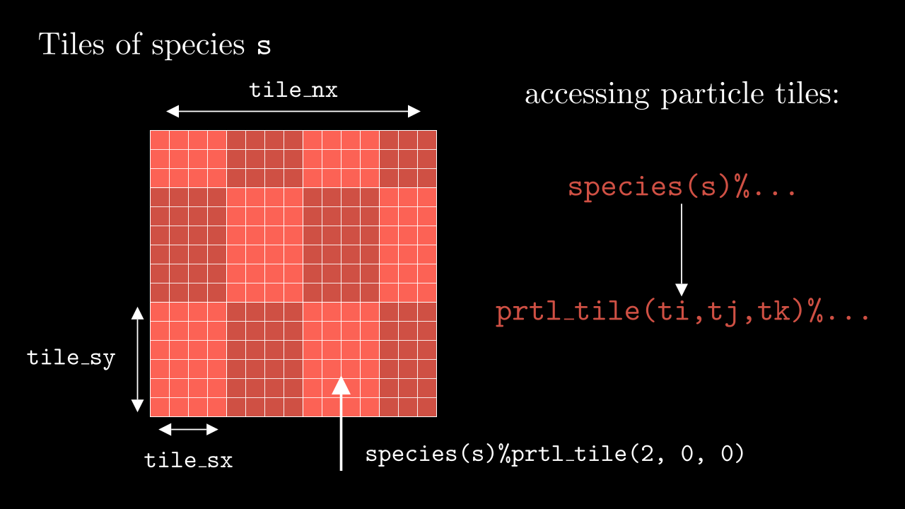
Particles in this code are stored as separate arrays within a tile, i.e., their positions and velocities are stored as separate arrays xi(:), dx(:), u(:), ... (so-called structure of arrays).
To access a particle we first need to access the particular species s, then address to the particular tile through its three dimensional index ti, tj, tk and then address to a particle property through its index p (see image below). E.g., a typical way of addressing would look like the following:
species(s)%prtl_tile(ti, tj, tk)%xi(p)
...%maxptl_sp that a particular tile can carry. This is done in src/logistics/exchange_particles.F90 in exchangeParticles() subroutine at the same time as the sending between MPI domains is taken care of.Coordinates of the particle in each direction are stored as two separate arrays. In x they are xi(:) and dx(:), where xi(p) is the i index of the cell where particle lives, and dx(p) is the displacement from the edges of that cell (see image below).
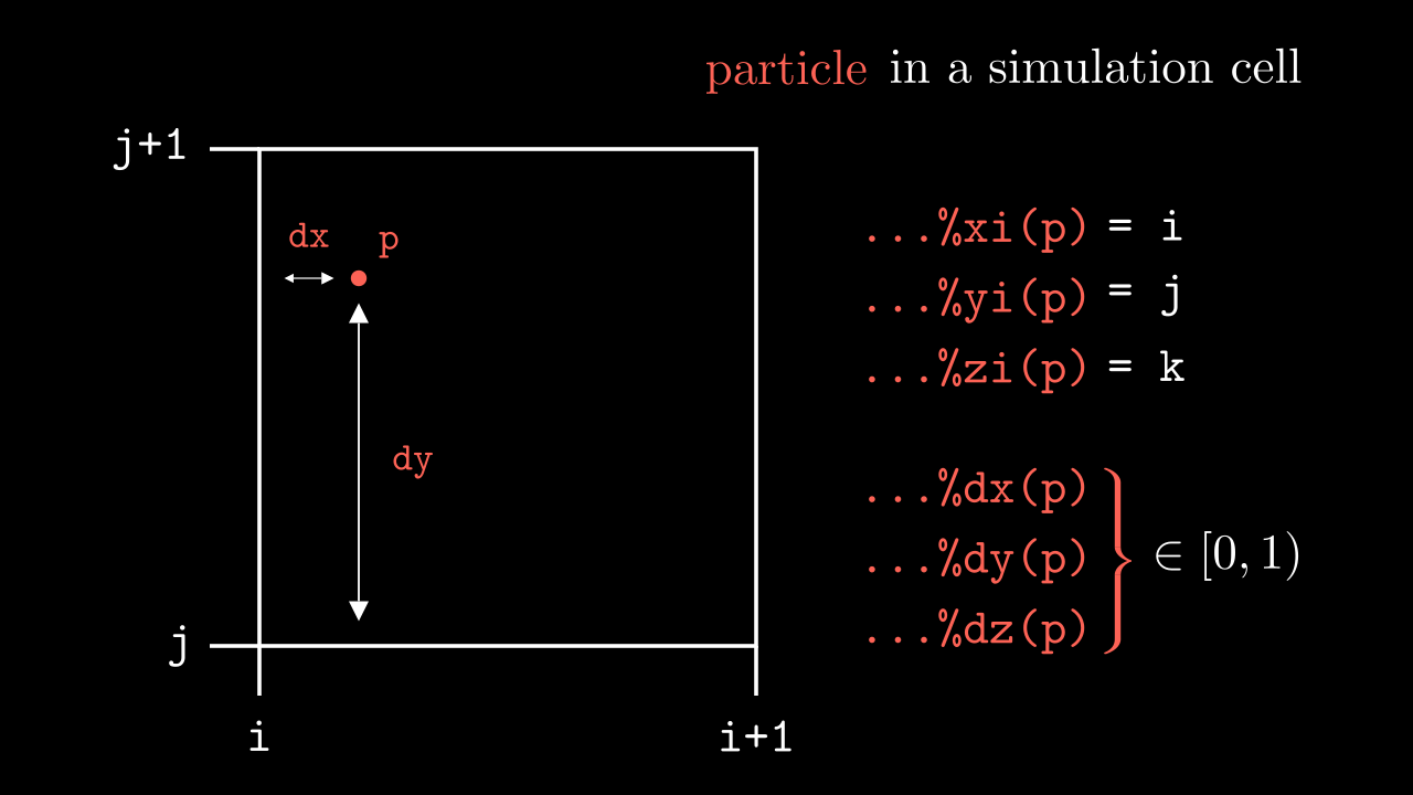
u(:), v(:), and w(:) arrays. So the energy of such a particle (in units of $m c^2$) can be found as sqrt(1 + u(p)**2 + v(p)**2 + w(p)**2). In case of massless particles, in the same arrays we store three components of their 4-momentum, meaning that their energy is sqrt(u(p)**2 + v(p)**2 + w(p)**2).Usage example
A typical loop over all particles of all species will look like this.
do s = 1, nspec ! loop over species
  do ti = 1, species(s)%tile_nx      ! loop over tiles in x
    do tj = 1, species(s)%tile_ny    ! loop over tiles in y
      do tk = 1, species(s)%tile_nz  ! loop over tiles in z
        do p = 1, species(s)%prtl_tile(ti, tj, tk)%npart_sp ! loop over particles in that tile
          ! getting global `x` coordinate of the particle `p` (notice adding `x0`)
          x_glob = REAL(species(s)%prtl_tile(ti, tj, tk)%xi(p) + this_meshblock%ptr%x0)&
                 & + species(s)%prtl_tile(ti, tj, tk)%dx(p)
          ...
        end do
      end do
    end do
  end do
end do