Unit normalization
For details see the following section.
Binary vs Monte-Carlo coupling
To simulate “two-body” processes, i.e., quantum interactions of two macro-particles, it is first crucial to invent a proper pairing routine that will loop through the particles within a given region, randomly pair them together, compute the corresponding interaction cross sections and then decide to either proceed with the interaction or not.
There are two approaches one can employ. We can either loop through all the possible pairs in a given region; in general this requires N^2 operations, where N is the number of particles in that region. This approach, while being the physically “correct” one, is extremely time-consuming. On the other hand, we could pair random particles in a given region only once at a given timestep, which can be done in O(N) operations. In our code we implement both approaches and then compare their performance and convergence. Also keep in mind, that there are two general scenarios that may occur: particles from group A may be interacting with particles from group B, or alternatively particles from the same group may be interacting with each other. Our generic coupling routines work with both of these situations.
MC pairing
In this subsection we will briefly describe the generic pairing routine that we employ in the code. This routine is written in such a way, that it can be implemented to simulate two-photon (Breit-Wheeler) pair-production, or Compton scattering, or Coulomb scatterings, or any other kind of binary interaction.
Tristan-MP v2 is an intrinsically multi-species code. In certain situations species can represent physical differences between the macro-particles (e.g., electrons, positrons, ions, photons etc), as well as conceptual differences (e.g., electrons injection to the simulation by user vs electrons produced from QED processes). Because of this the pairing routine has to be agnostic to species, and only pair the two groups of particles (to whatever species they belong).
In the src/tools/binary_coupling.F90 we can find the coupleParticlesOnTile() subroutine which pairs two particle groups on a single tile. Let us quickly go through the arguments this function accepts.
(in) ti, tj, tk- tile indices;(in) sp_arr_1, n_sp_1- array of species for the groupAof particles, as well as the number of species (not particles) in that array;(in) sp_arr_2, n_sp_2- same for the groupB(notice, these values forAandBcan be equal);(out) coupled_pairs, num_couples- returned randomcouplesof pairs from groupsAandB, and their number;(out) num_group_1, num_group_2- returned number of particles in each group.(out) wei_1, wei_2- returned total weight of particles in each group.
Returned couples are types of objects defined in the following way:
type :: spec_ind_pair
  ! object which identifies a particle ...
  !     ... by its species and index on a given tile
  integer :: spec, index
  real    :: wei ! particle weight
end type spec_ind_pair

type :: couple
  ! object that contains two particles ...
  !     ... given by their species and index ...
  !     ... on a single tile
  type(spec_ind_pair) :: part_1
  type(spec_ind_pair) :: part_2
end type
So to extract from memory the (x coordinate of the) first particle from one of the returned couples, one would do:
sp = couple%part_1%spec
pp = couple%part_1%index

species(sp)%tile(ti, tj, tk)%x(pp)
Remember, that any particle can be uniquely identified by the corresponding tile indices (ti, tj, tk), the species index (s) and its own index (p).
The subroutine can pair particles with arbitrary weights. For particles with weight larger than the reference weight of 1, we split the total weight evenly among CEILING(weight) copies of the particle. This improves the MC sampling for heavy particles, which can carry a large fraction of
the total group weight but would be accounted for only crudely if they are not split into order-unity weight particles. This pairing algorithm for just two “heavy” particles is illustrated in the animation below. Similarly one can do grouping of two or more particles by splitting them within each group and treating them as individual light particles.
coupleParticlesOnTile() only make couples from the given particle groups, it doesn’t handle the consequent physics that should be carried on these particle couples later.Breit-Wheeler pair production
Theory
Breit-Wheeler process is a pair production mechanism that transforms two high energy photons into an electron-positron pair. This process can proceed if the energy of two photons in their common center-of-momentum frame is larger than $2m_e c^2$:
where $\varepsilon_1$ and $\varepsilon_2$ are the energies of two photons, and $\theta$ is the angle between their momentum vectors in the lab frame.
Quick user guide
To enable the Breit-Wheeler pair production one must first add the following two flags when configuring the Makefile: -qed, -bwpp. In the input file this module requires several parameters to be included:
<bw_pp>

  tau_BW        = 0.01          # fiducial optical depth
  interval      = 1             # perform BW once every `interval` timestep
                                # ... this value renormalizes the cross section,
                                # ...... so no need to worry about changing the `tau_BW`
  algorithm     = 1             # 1 = BINARY; 2 = MC
  electron_sp   = 3             # save produced electrons to species #...
  positron_sp   = 4             # save produced positrons to species #...
Additionally we must define two species in the <particles> block of the input that would be treated as electrons/positrons:
  maxptl3       = 1e6           # max number of particles per core
  m3            = 1
  ch3           = -1

  maxptl4       = 1e6           # max number of particles per core
  m4            = 1
  ch4           = 1
And of course let’s not forget about the photons themselves:
  maxptl1       = 1e6           # max number of particles per core
  m1            = 0
  ch1           = 0
  bw1           = 1

  maxptl2       = 1e6           # max number of particles per core
  m2            = 0
  ch2           = 0
  bw2           = 2
Notice the bw1 and bw2 parameters. The fact that they’re different means the algorithm will be treating these as two separate groups of photons interacting with each other: photons from group #1 interact with photons from group #2, but not with the photons from the same group. Alternatively we could have only one group of photons interacting with themselves:
  maxptl1       = 1e6           # max number of particles per core
  m1            = 0
  ch1           = 0
  bw1           = 1

  maxptl2       = 1e6           # max number of particles per core
  m2            = 0
  ch2           = 0
  bw2           = 1             # <-- same group now
… or like this (if the second photon species is unnecessary):
  maxptl1       = 1e6           # max number of particles per core
  m1            = 0
  ch1           = 0
  bw1           = 1
Implementation details
In our simulations this process takes place in every simulation tile separately. Particles (with arbitrary weights in general) in each tile are paired using either the Monte-Carlo pairing discussed above or using a brute force binary pairing. This process provides us with pairs of abstract particles with weights $\sim 1$.
For each of these pairs we first compute the $s$-parameter to find out whether these particles can in principle pair produce, and after that we compute their interaction cross section which is a function of $s$ (see the full expression in Akhiezer & Berestetskii (1965) QED). This cross section, normalized to the tile size, BW interval and the fiducial number specified in the input, serves as a criterion for the particles to either pair produce or not. If it is decided that two particles shall pair produce – we compute the weights, energies and momenta of produced electron and positron according to the differential cross section (in the C-o-M frame) in such a way, that the weight, energy and all momentum components are conserved. We then generate a random position in the tile where we initialize the two charged particles and subtract the corresponding weights from the original photons (if the photon “spends” all of its weights – we destroy it, and it may not further participate in this process).
ppc0 or decrease tau_BW.Tests
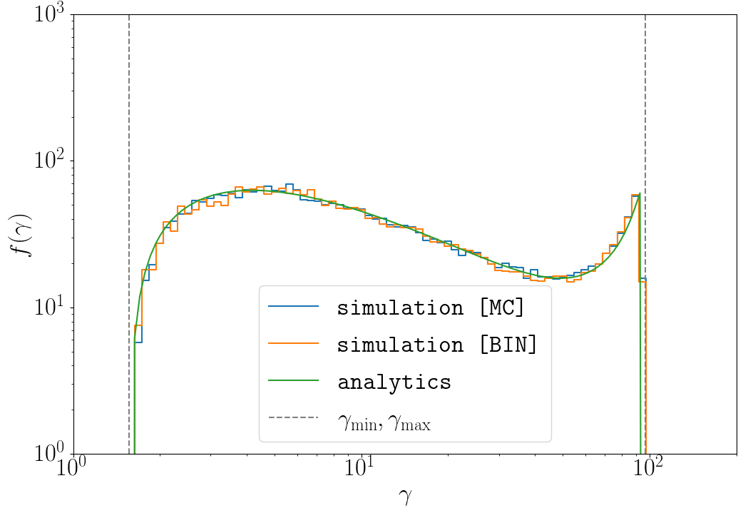
Depending on which algorithm is chosen, the routine goes through some procedure and produces electron/positron pairs respecting the computed differential cross section. The total energy and momentum (of two photons before the process, and of the pair after the process) is exactly conserved.
On the plot below we compare the two pairing methods (binary and Monte-Carlo) with the analytic model from Aharonyan+ 1983. We initialize a periodic box with two isotropically distributed monoenergetic photon populations with energies $\varepsilon_1 = 0.1 m_e c^2$ and $\varepsilon_2 = 100 m_e c^2$.
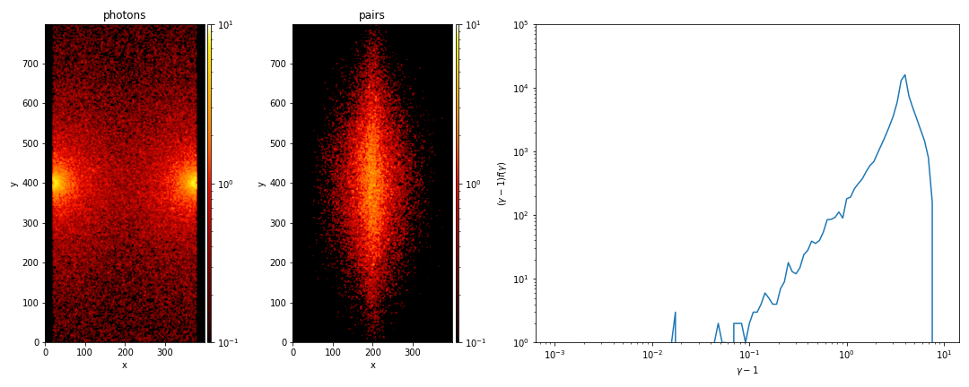
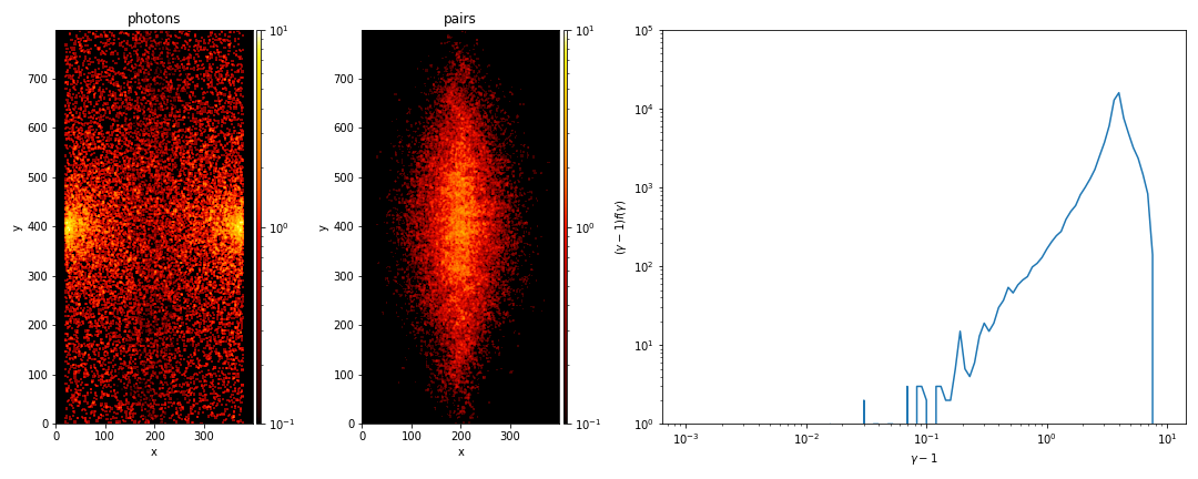
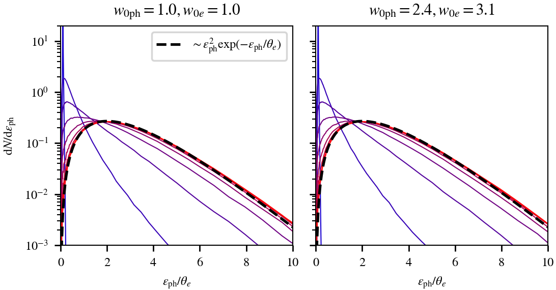
Pair production process respects particle weights. This means that (in an ideal situation) there should be almost no difference between two-photon pair production of two macro-photons with weights 1 and 10, and between 11 separate macro-photons. However, of course, there is no free lunch, so downsampling, as expected may reduce the sampling resolution of the photon distribution function, and, as a result, the distribution function of produced electron-positron pairs.
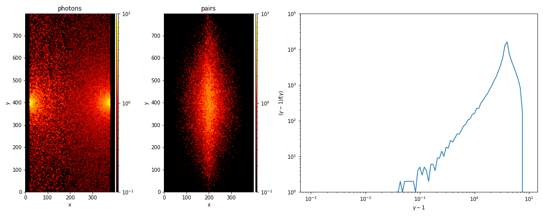
Below we present an example simulation where we initialize two monoenergetic photon sources, with energies $E\sim 5 m_e c^2$, emitting two counterstreaming photon populations at a given rate. We present 3 cases with varying weights of emitted photons, the rates are adjusted accordingly. The leftmost panel in all 3 cases is the photon number density, the central panel is the density of produced pairs (which for the purposes of demonstration are frozen), and the rightmost panel is the spectrum of produced pairs.
Compton scattering
Quick user guide
To include support for Compton scattering,
run the Makefile configuration script with the -qed and -compton flags.
The main functionality can be controlled with the parameters in the
<compton> block of the input file:
<compton>

  tau_Compton   = 0.01     # fiducial optical depth
  interval      = 1        # scatter once every `interval` timesteps
  algorithm     = 2        # 2 = MC; binary is currently not supported
  el_recoil     = 1        # enable the recoil on the electron in the scattering
  Thomson_lim   = 1e-5     # photon energy in the electron rest frame...
                           # ... below which the scattering is done in the...
                           # ... Thomson regime
Particles belonging to some species 1 will participate in the scattering
if their compton1 parameter is configured:
  maxptl1       = 1e6           # max number of particles per core
  m1            = 0
  ch1           = 0
  compton1      = 1             # enable Compton scattering
The list of Compton-enabled species has to include at least one electron/positron and one photon species. Ions cannot participate in the process.
Implementation details
The implementation details are similar to those described in Del Gaudio+ 2020 with a few variations. Central to the model is the calculation of an appropriately normalized scattering cross section for every electron-photon pair and the random sampling of the photon scattering angle in the electron rest frame. The differential Klein-Nishina cross section for unpolarized photons in the electron frame reads (see, e.g., Berestetskii+, Quantum Electrodynamics (Pergamon, Oxford, 1982)):
where $u = \cos\theta’$ is the cosine of the scattering angle (i.e., the angle between the initial and scattered photon direction in the electron frame), $\sigma_{\rm T}$ is the Thomson cross section, and $\rho$ is the ratio of the scattered to initial photon energy in the (primed) electron rest frame:
Here $\epsilon_{0,1}’ = \hbar\omega_{0,1}’ / m_ec^2$ is the normalized energy. The total cross section (integrated over $u$) can be written as
For the random sampling of $u = \cos\theta’$ we make use of the cumulative probability distribution similar to Del Gaudio+. The cumulative distribuion can be expressed as
where
To obtain a random cosine $u$, we select a random number $R\in[0,1)$ and solve iteratively (via a Newton root find) for ${\rm CDF}(u) = R$. The coefficients ${c_i}$ can be computed only once per every root find. Convergence is typically achieved in only a few iterations. For $\epsilon_0’\ll 1$ we expand ${\rm CDF}(u)$ to 2nd order in $\epsilon_0’$ to avoid numerical issues with evaluating the full expresion in this regime.
The (Monte-Carlo) scattering algorithm works as follows. We first construct random electron-photon pairs on every tile. For each pair from the list, the photon momentum and energy are transformed into the electron (or positron) rest frame:
where $\boldsymbol p_0$ is the electron momentum and $\boldsymbol k_0$ is the initial simulation-frame photon momentum (both in units of $m_e c$). Once in the rest frame, the electron-photon pair is scattered with probability
where $\tau_{\rm T}$ is our fiducial Thomson scattering optical depth (as measured in code units; $\Delta t = \Delta x = 1$), $\hat \sigma = \sigma(\epsilon_0’)/\sigma_{\rm T}$ is the total Klein-Nishina cross section in the electron rest frame normalized to $\sigma_{\rm T}$, and $P_{\rm corr}$ is a probability correction/normalization factor that accounts for variable numbers of particles on a tile, particle weights, etc. (see details below). The factor $\epsilon_0’/\epsilon_0\gamma_0$ transforms the probability from the rest frame into the simulation frame. It is worth noting that this last term not only adjusts the total probability but also assigns a different probability to each saparate scattering, depending on the momentum of the photon and electron.
tau_BW and tau_Compton parameters should be actually the
same because both cross sections are normalized to $\sigma_{\rm T}$.Once an electron-photon pair is selected for scattering, we pick a random scattering cosine as described above, update the photon momentum (projecting different components of $\boldsymbol k_1’$ onto an orthogonal basis) and Lorentz boost back into the simulation frame. The momentum of the scattered electron in the simulation frame is finally obtained via momentum conservation: $\boldsymbol p_1 = \boldsymbol p_0 + \boldsymbol k_0 - \boldsymbol k_1$
Normalizations
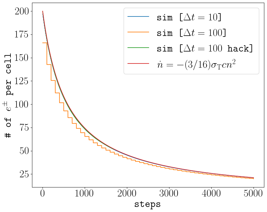
Several aspects need to be taken into account for an appropriate normalization of probabilities: (i) the time evolution should be independent of numerical parameters such as number of particles per cell, time step, particle weights, and (ii) the MC pairing should match the full binary pairing. Below we describe the normalization step by step.
First, the probability should be independent of the number of particles per cell, tile size, and time step. This gives as a starting point:
where $n_{\rm ppc}$ is the number of particles per cell, $s_x$, $s_y$, $s_z$ are the tile sizes in cell units, $\Delta t_C$ is the time step for Compton scattering, and $\Delta t$ is the PIC loop step. By normalizing with the reference number of particles per tile, the physical density is effectively set with the choice of the optical depth $\tau_{\rm T}$. Note: If the number of particles per tile increases above the (fixed) reference value during simulation the probabilities do increase accordingly.
Next, we consider the matching of probabilites with full binary pairing. In the case of MC, each (split) particle can interact with at most one particle from the other group. In reality, all possible interactions should be considered. To account for this, the probability needs to increase:
where $w_1$ and $w_2$ is the total weight of particles in group 1 and group 2, respectively.
Finally, we mention the implications of pairs with non-equal weights. Without counting particles twice, at most $\min(n_1, n_2)$ pairs can be generated, where $n_1$ and $n_2$ are the total numbers of particles in each group. It is important to notice that the total weight of particles which have been paired may be significantly less than the the total weight of both groups. Furthermore, it may not be possible to scatter the total portion of the paired weight. If the weights in a given pair ($w_{1i}$, $w_{2j}$) are unequal, the weight of the lighter particle needs to be split away from the heavier one, and only the split portion is scattered (see Haugbolle+ 2013, Del Gaudio+ 2020) . To account for these circumstances, the probability needs to be adjusted:
Here, the numerator represents the amount of weight that could be scattered in an ideal situation, while the denominator is the amount that can be actually scattered. All the probability corrections can be now combined into the final expression:
Tests
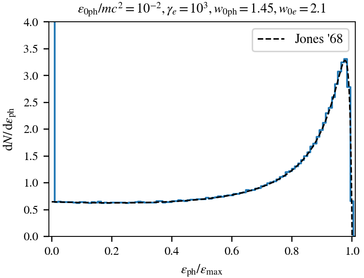
Using the above-described algorithm, we perform a series of common tests. This includes the Comptonization of soft photons in a thermal electron background (Kompaneets 1957) and the spectrum of isotropic photons scattered off a relativisic electron (Jones 1968). The results agree well with theory. We also perform the tests with unequal initial electron and photon weight. This leads to the splitting of particles. The physical results are unaffected by such choice and remain in excellent agreement with the case where all weights are 1.
Pair annihilation
Quick user guide
To enable the pair annihilation we must first add the following two flags when configuring the Makefile: -qed, -annihilation. In the input file this module requires several parameters to be included:
<annihilation>

	interval			= 1							# perform pair annihilation every `interval` timestep [1]
	photon_sp			= 3							# produced photons are saved to species #... [3]
	sporadic      = 0							# enable/disable sporadic annihilation for interval > 1 [0]
sporadic enables randomization of this process in time for each tile if the interval is greater than 1.
We may then enable this process for particle species:
<particles>

  nspec         = 3             # number of species [2]

  maxptl1       = 1e6           # max # per core [*]
  m1            = 1             # mass (in units of m_e) [*]
  ch1           = -1            # charge (in units of q_e) [*]
	annihilation1 = 1							# species can participate in pair annihilation [0]

  maxptl2       = 1e6
  m2            = 1
  ch2           = 1
	annihilation2 = 1

  maxptl3       = 1e6
  m3            = 0
  ch3           = 0
The list of species has to include at least two species with opposing charges and equal masses.
Tests
A simple setup that tests all the QED modules coupled together is described in Beloborodov (2020), where we initialize a thermal \(e^\pm\) distribution and enable all three of the QED processes: pair-production/-annihilation and Compton scattering. Pairs annihilate producing photons, photons upscatter on pairs, and the highest energy ones produce new pairs. The result is that we form a Wien distribution in photons and a corresponding thermal distribution in pairs with the same temperature.