Synchrotron cooling
To enable synchrotron cooling add the following flag during the configuration: --radiation=sync. This will enable the synchrotron drag force and the instantaneous photon spectrum. To also create physical photons tracked in simulation as regular particles add the -emit flag.
Notice that you should also specify the following parameters in the input file (will describe them below):
<radiation>
  gamma_syn      = 10.0          # determines the synchrotron cooling rate
  emit_gamma_syn = 50.0          # determines synchrotron photon peak energy
  beta_rec       = 0.1           # fiducial number that goes into the definition of `gamma_syn`
  photon_sp      = 3             # emit photons to species #...
  dens_limit     = 1000000       # density limit on the cooled region
photon_ind is the species index of photons, to which the synchrotron photons will be added. dens_limit is the maximum cell density (computed as a sum of all massive particle species) where the cooling is turned ON (i.e., when rho > dens_limit the cooling is OFF).
The cooling can also be turned on or off for a particular particle species through the input file.
<particles>
  cool1          = 1            # turn the cooling ON for species #1
  cool2          = 0            # turn the cooling OFF for species #2
Synchrotron radiation drag
Radiation reaction force for a particle with a 4-velocity $\boldsymbol{u}=\gamma\boldsymbol{\beta}$ is given by the following expression:
where $r_e$ is the classical electron radius, $B_{\rm norm}$ is the electric/magnetic field normalization, and $\boldsymbol{\kappa}_R$ and $\chi_R$ are dimensionless functions of $\boldsymbol{\beta}$ and electric/magnetic fields:
It is useful to parametrize this relation with the parameter, $\gamma_{\rm syn}$ (read as gamma_syn in the input). The physical meaning of this parameter is the following: a particle with $\gamma=\gamma_{\rm syn}$ in the magnetic field of $B=B_{\rm norm}$ experiences a radiation reaction force, equal to the acceleration by an electric field $E=\beta_{\rm rec} B_{\rm norm}$ ($\beta_{\rm rec}$ is some fiducial magnetic energy extraction rate):
This dimensionless parameter basically upscales the classical electron radius and defines the synchrotron cooling rate. We can thus rewrite the particle equation of motion under the radiation drag as the following
|e| == m_e.Photon emission
Now we might also want to know what the radiated photon spectrum looks like. For that we need a way to take the radiated energy subtracted by the radiation reaction force and deposit it to photons (either real photon particles or just into spectrum).
We will assume that at each moment in time particle can only radiate a photon with the corresponding synchrotron peak energy. For that we need another dimensionless parameter, $\tilde{\gamma}_{\rm syn}$ (think of \tilde as of photon :)), which determines the Lorentz-factor of a particle that in the magnetic field $B = B_{\rm norm}$ has a synchrotron peak equal to the particle rest mass energy, $m_e c^2$:
This dimensionless parameter basically sets the scale of $\hbar$ in our simulation units. For the peak energy of synchrotron photons we thus have:
While the radiation drag will be applied continuously at every timestep, we will radiate a photon with a certain probability, $p_{\rm ph}$, to satisfy the following condition on the overall cooling rate:
from which we find that:
If the photon emission is enabled, i.e., if we create photons as simulation particles, we will continuously apply the radiation reaction force and create a photon with energy $\varepsilon_{\rm ph}$ with a probability $p_{\rm ph}$. If the emission is turned off, we can still track the instantaneous radiation spectrum by depositing $p_{\rm ph}$ into the spectral bin corresponding to $\varepsilon_{\rm ph}$.
spec = isolde.getSpectra('spec.tot.*****') you can access the instantaneous radiation spectrum (separate for every species) even if the photon emission was turned off: spec['r1']['bn'] and spec['r1']['cnt'] for the radiation from species #1.Physical intuition and numerical tests
Since these $\gamma_{\rm syn}$ and $\tilde{\gamma}_{\rm syn}$ parameters can become annoyingly counter intuitive, here is a good way to think about them. While $\sigma$ together with the skin depth, $c/\omega_{\rm p}$, and $n_{\rm ppc}$ set the value of the magnetic field $B_{\rm norm}$, $\gamma_{\rm syn}$ and $\tilde{\gamma}_{\rm syn}$ rescale the values of the so-called classical magnetic field $B_{\rm cl} = m_e^2 c^4/e^3$ and the Schwinger magnetic field $B_{\rm S} = m_e^2 c^3 / e\hbar$ (effectively rescaling the Thomson cross section and Planck’s constant). In fact, we can express these parameters in the following way
where $\alpha$ is the fine-structure constant $\approx 1/137$.
Inverse Compton cooling
To enable inverse Compton cooling add the following flag during the configuration: --radiation=ic. This will enable the IC drag force and the instantaneous photon spectrum. To also create physical photons in the simulation add the -emit flag.
Same as for the synchrotron, you should also specify the following parameters in the input file (will describe them below):
<radiation>
  gamma_ic       = 20            # determines the cooling rate
  emit_gamma_ic  = 10            # determines the peak energy
  beta_rec       = 0.1           # fiducial number that goes into the definition of `gamma_ic`
  photon_ind     = 3             # index of species to which to emit photons (if `-emit` is ON)
  dens_limit     = 100           # density limit on the cooled region
Just as in the previous section, photon_ind is the species index of photons, to which the synchrotron photons will be added. dens_limit is the maximum cell density (computed as a sum of all massive particle species) where the cooling is turned ON (i.e., when rho > dens_limit the cooling is OFF).
The IC cooling can also be turned on or off for a particular particle species through the input file.
<particles>
  cool1          = 1            # turn the cooling ON for species #1
  cool2          = 0            # turn the cooling OFF for species #2
IC radiation drag
The drag on a relativistic particle in an isotropic soft radiation field with energy density $U_{\rm ph}$ is given by
where $\sigma_T = (8\pi/3) r_e^2$ is the Thomson cross section. We assume that the
Klein-Nishina effect is negligible, although this would only add
a multiplicative factor to the scattering cross section.
Similar as for synchrotron cooling, we introduce a characteristic Lorentz factor $\gamma_{\rm IC}$ (named gamma_ic in the input file), which characterizes the cooling
strength. This is defined by balancing the inverse Compton cooling against the acceleration from a fiducial reconnection electric field:
In the new parametrization, the IC drag reads
IC photon emission
When emission is switched on, particles may randomly emit photons with energy equal to the IC peak energy. The peak energy of the upscattered photons is $\varepsilon_{\rm ph}\approx \gamma^2\varepsilon_{0},$ where $\varepsilon_{0}$ is the energy of the soft photons before scattering. Instead of using $\varepsilon_0$ we introduce
(parameter emit_gamma_ic in
the input file), which gives the particle Lorentz
factor required to emit a photon with energy $m_ec^2.$ The IC photon energy can be
therefore written as
Same as for synchrotron emission, we introduce the emission probability $p_{\rm ph}$, which is found at every step and for every particle via momentum conservation. That is, we require that the change of particle momementum due to the IC drag is equal (in a statistical sense) to the momentum of the newly emitted photons:
This gives the emission probability at a given timestep:
Numerical tests
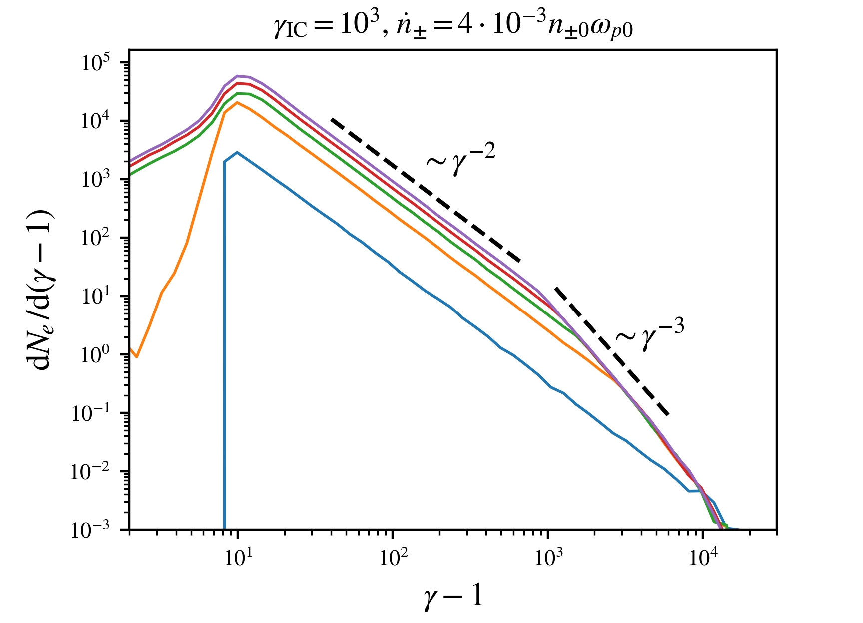
One astrophysically relevant test is a radiatively cooled plasma where particles are continuously injected by sampling from a power-law energy distribution. In the test below, we study the evolution of the electron energy spectrum in the presence of such continuous injection and IC cooling. The injected particles have a $p=-2$ energy spectrum exponent. As theoretically expected, the energy spectrum develops a cooling break with a spectral exponent of $p-1$. The break shifts to ever lower energies over time.